Abstract

In this laboratory exercise, various characteristics of open channel fluid flow were investigated in a variety of experimental setups. Different characteristics including hydraulic jumps and their associated energy losses, flow around sharp and curved bodies, spillways, weir-based flow rate measurement techniques, as well as fluid jet projections from orifices on vertical columns of water were observed.  Measured data values were then compared with theoretical models.

 

Introduction

In this lab, different methods were used to quantitatively analyze open channel flow.  In the first part of the lab, the Froude number and its relation to rapid (or tranquil) were observed and the energy losses associated with different flows were calculated. 

      In the spillway analysis, the Bernoulli equation and the concept of conservation of mass were used to derive final velocities and the energy losses of the system in various flow rates.

      For the weir flow analysis, the water flow over a 60º weir was observed and the theoretical flow rates were calculated using the height drop of water above the notch.

      In the next part of this lab, fluid jet projection from an orifice was observed and the results were compared to theoretical results obtained using the Bernoulli equation.

      For the final part, the waves generated by solid bodies in an open channel flow, the turbulent flow around the obstacles and the flow around different obstacles were observed and compared.

 

Procedure

See attached handout.

 

Theory, Results and Discussion by Experiment

 

Hydraulic Jump

 

Hydraulic Jump Theory

A hydraulic jump is a step upwards in the elevation of a free surface in open channel flow. The Froude number represents the ratio of inertial to gravity forces acting on a flow, defined as. When the Froude number is greater than one, the flow is rapid or supercritical, and when it is less than one, the flow is tranquil or sub-critical. When the fluid undergoes a hydraulic jump, the flow is supercritical upstream of the jump and sub-critical downstream of the jump. Hydraulic jumps are typically intensely turbulent and can be effective energy dissipaters.

 

 

 

 

 

Figure J1.

 

Hydraulic Jump Results

Froude numbers and Reynolds numbers were calculated both at the entrance to the channel before the jump (position 0) and at a point after the jump (position 1).

 

Table J1. Hydraulic Jump Characteristics at Each Flow Rate

% flow	h1/h0	Fr0	Fr1	Re0	Re1	%KE lost
69	12.09	20.05	0.4766	3530	3500	93.3
51	6.61	14.88	0.8751	2620	4760	91.8
30	5.96	8.85	0.6069	1560	3130	82.4

 

Hydraulic Jump Discussion

The flow loses most of its energy at the hydraulic jump, especially at high flow rates. The flow has lost nearly all its kinetic energy and only increased its average height by a small amount, corresponding to a small gain in potential energy. The Reynolds numbers show that the flows should all be turbulent or nearly turbulent at position 1, after the jump. The Froude numbers at this point, however, indicate a sub-critical flow. The Froude numbers at position 0 correspond well with those expected from the ratio of the heights before and after the jump, according to the text.[1] The surprisingly high percentages of energy lost could be explained by the fact that the calculations only include the kinetic energy of translational motion. All of the energy of rotation associated with the turbulent flow indicated by the Reynolds numbers is not factored into the total kinetic energy in the calculations, so it is considered lost. The discrepancy between the large Reynolds numbers after the jump (indicating turbulence) and the sub-critical Froude numbers there (indicating tranquil flow) may be explained by the position of the plate at the end of the channel. The theory assumes that the region after the jump is very large compared to the jump region, so that effects of the boundaries should be negligible. The effects of the plate, however, are clearly not negligible, since measurements were taken only inches away from it, and turbulence was still present.

 

Waves Generated by Sharp Bodies

 

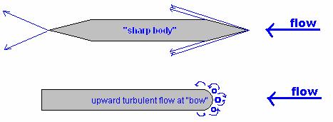
Waves were generated by the sharp bodies upon their immersion into the open channel flow.  As clearly seen in figure B1, the sharp body creates defined transverse flows in nearly the same angles as the point of the body.  Transverse flows also emerge at the tail end of the body, at the same angles at the transverse flow created at the bow.  For the body with a rounded end, turbulent flows arise as the fluid creeps up vertically on the body.  The fluid should ideally reach the height of the spillway off which it came, but due to considerable losses, the fluid barely managed to peak over the top of the body before reaching zero vertical velocity and returning downwards.  This fact has large implications for bridges and piers, due to the large stresses at the base and the resulting erosion.

 

Figure B1. Open Channel Flows Around Obstructions

 

 

 

Spillway

 

Spillway Theory

 

Energy analysis of flow in an open channel can be performed using the Bernoulli’s equation with losses, which follows:

(1)                   

This equation can be further simplified by accounting for the variation in the height of the bottom of the channel, , as part of the losses.  Additionally, due to the near hydrostatic pressure for any cross section of the flow, it can be assumed that  and , where y is the height above the .  The resulting energy equation is as follows:

(2)                   

If the flow rate of the fluid in the channel is known, fluid velocity analysis for flow over the spillway can also be performed using the conservation of mass equation at steady state, .  Since water can be assumed to be an incompressible fluid for this experiment, we can assume that water maintains a constant density.  As such, we can assume conservation of volume which is characterized by the following equation for flow through a control volume at steady state:

(3)                   

Where,

         Q is the volumetric flow through the channel

V_i is the velocity when x=i

A_i is the area of the cross section at x=i

Estimates for the losses can then be found by combining equations 2 and 3 into the following form:

(4)                   

Figure S1.

 

Spillway Results

 

The observed depths of water at a point upstream, at the crest of the spillway, at the foot of the spillway, and at a point downstream, see figure S1, are recorded in table S1.

 

Table S1. Observed Depths and Cross-Sectional Areas

at Four Points Along the Spillway Channel

 

Using the conservation of volume at steady state and the known calibration coefficients to determine the flow rate in the channel, the fluid velocities at a point upstream, at the crest of the spillway, at the foot of the spillway, and at a point downstream were calculated.  The results of these calculations have been recorded in table S2.

 

 

 

 

Table S2. Velocity Calculations Based on Conservation of Mass

and Rotameter Flow Rates

 

Energy analysis was then performed using Bernoulli’s equation with losses to determine the energy lost between consecutive states.  The resulting losses have been recorded in Table S3.  The inconsistent foot velocity and loss estimations for the 70 percent rotameter flow results from the measurement of the height at the foot of the spillway.  If the measurement had continued the trend established between the 30 and 50 percent tests, the depth of the water would have increased by 0.04 inches from 0.11 to 0.15 inches.  With this adjustment, the loss estimates would have been 5.22 and 0.90 inches of water, which are both inline with the 30 and 50 percent estimates.  Results for data with the adjusted height at the foot have been recorded in all tables as 70 percent adjusted.

 

Table S3. Head Loss estimates based on Bernoulli’s with Losses

and Rotameter Velocity Calculations

Using the Bernoulli’s equation, the loss estimations, and assume that the fluid velocity upstream of the spillway is approximately zero, estimations of the velocities at the crest, foot, and downstream were calculated.  The resulting values are recorded in Table S4.

 

Table S4. Velocity Estimations using Energy Analysis and Estimated Losses

 

Performing mass conservation analysis on the results from the energy analysis lead to estimations of the flow rate, which can be compared to the rotameter values for error analysis.  The resulting flow rate estimates have been recorded in table S5.

 

Table S5. Flow Rate Estimates From Energy Analysis Results

 

Froude numbers were calculated for the water at the crest of the spillway, foot of the spillway, and downstream from the spillway.  The results have been recorded in Table S6.

 

Table S6. Froude Numbers

 

Spillway Discussion

 

As previously mentioned in the spillway results section, it appears that the measurement of the depth of water at the foot of the spillway during the 70 percent test run was improperly measured or recorded, as the values resulting from the adjusted thickness were consistent with the 30 and 50 percent test runs.  From the results, the head loss drop due to the drop over the spillway was approximately 5.2 inches.  The losses between the foot of the spillway and downstream were identified both by observation and calculation to be due to hydraulic jumps.  The analytical evidence of the hydraulic jump in the fluid between the foot and downstream is the supercritical Froude numbers at the foot and subcritical Froude numbers downstream.  Since the depth of water, with the exception of the upstream data, was less than a quarter inch, the assumption, that the velocity profile was uniform, was valid. 

 

Weir Flow Analysis

 

Weir Theory

According to the text, the volume flow rate over a weir is given by

where θ is the angle of the weir (for our setup θ = 60º), H is the height of the flow before the weir with respect to the weir notch, and k is a constant factor[3]. Values of k were calculated from the data for each flow rate. An average of these k values (k_avg = 0.31167) was then used to calculate theoretical flow rates from the height measurements.

 

Figure W1.

 

Weir Results and Discussion

Table W1. Experimental and Theoretical Flow Rates over a 60^o Weir

Flow Setting	QExperimental	Associated k	QTheoretical	Error in Q
70%	0.015319	0.306667	0.015569	1.63 %
50%	0.011368	0.320091	0.011069	2.63 %
30%	0.006759	0.308239	0.006834	1.11%

 

The minimal errors can be attributed to measurement uncertainty. The equation given above does not, however, consider the effects of lateral flow. Flow in from the sides and particularly up from the bottom of the channel were visible during the experiment with the aide of dye, and both would act to increase the actual rate of flow through the weir.

 

Fluid Jet Projection from an Orifice

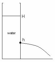
A column of water with a small hole projects a stream of water.  The orifice is installed at some height h from the baseline, and the top of the water column is at height H.  The horizontal projection of the stream was measured at various column heights.  From these measurements, the initial jet velocity was calculated.  Theoretical values were also calculated, and the results are shown below.  That the measured values are all slightly less than the theoretical ones can be readily accounted for by frictional drag losses not accounted for in the theoretical model.

 

Theory

 

Writing Bernoulli’s equation for a point at the top of the water column and right outside the orifice, we get

Assuming no velocity at the top of the column, and equal (atmospheric) pressures at both points, the equation simplifies to

We can calculate the time it takes for the jet to hit the baseline.  Knowing the time, we can multiply by the initial horizontal velocity V₂ to get the horizontal distance the jet travels.  The equation relating the orifice height and time is

Solving for t, we get

Multiplying the time equation with the initial velocity equation yields the horizontal projection as a function of orifice height h:

We find the maximum horizontal projection as a function of the orifice height by solving

Differentiating, we get

 

which gives the optimal orifice height to be

 

Jet Results and Discussion

 

Table O1. Observed and Theoretical Projection Distance and Velocity of a Jet by Height H

 

Figure O1.

 

As shown in Figure O1, the measured and theoretical velocities correlate very well.

 

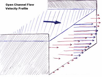
Velocity Profiles in Open Channel Flow

 

For an open channel flow of water in a rectangular channel, the maximum fluid velocity occurs at the center of the channel horizontally, slightly below the free surface.  The fluid adheres completely to the solid surfaces of the channel, causing the velocity distribution to be non-uniform.  As was observed in Lab 1, moving fluids experience a drag force at the free surface interface with the air, although the velocity does not go to zero as it does at a solid wall.  In Lab 2, internal laminar flow in a pipe resulted in a quadratic velocity profile.  In the horizontal direction, the problem would be reduced to internal flow problem with quadratic (or possibly higher even ordered polynomial) profiles. In the vertical direction, if there were no drag force at the surface, the velocity would increase from zero at the bottom to a maximum at the surface. The drag lowers the velocity at the surface though, and therefore that slightly below the surface as well. Thus, the maximum velocity of the channel flow can be found below the free surface in the center of the channel, as shown below.

 

 

For a uniform-depth open channel flow situation, the Manning equation can be used to calculate an average flow rate through a channel.  It is calculated from the wetted perimeter, area, and the channel’s incline. In the equation, R_h is the hydraulic radius, which is simply the cross-sectional area divided by the wetted perimeter.  S₀ is the slope of the channel, and n a empirical constant accounting for the channel surface material.

For the case where the depth of the flow y is half the concrete channel width b, R_h is

 

and the Manning equation simplifies to

where y is the flow depth, and n is replaced by the constant value for a smooth concrete channel.  This equation is very useful for designing irrigation systems and solving other uniform depth open channel flow problems.