Engineering 58 Pade Approximations, Aron Dobos, 26 February 2005

Contents

First order Padé approximation step response with MATLAB (Td = 1).

sys1st = tf([-1 2], [1 2]);

Second order transfer function.

sys2nd = tf([1 -6 12], [1 6 12]);

Inverse Laplace transforms of the step responses.

syms s;
pretty( ilaplace( (-s+2)/(s*(s+2)) ) )
pretty( ilaplace( (s^2-6*s+12)/(s*(s^2+6*s+12)) ) )

 
                                1 - 2 exp(-2 t)
 
                              1/2                1/2
                       1 - 4 3    exp(-3 t) sin(3    t)

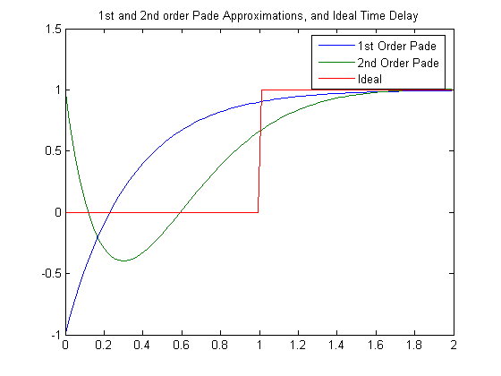
Plotting the responses

[y1 t] = step(sys1st);
[y2 t] = step(sys2nd);
y3 = heaviside(t-1);
plot(t, y1, t, y2, t, y3);
title('1st and 2nd order Pade Approximations, and Ideal Time Delay');
legend('1st Order Pade', '2nd Order Pade', 'Ideal');

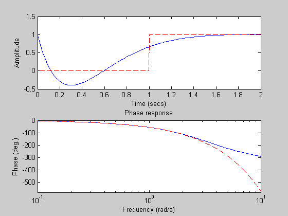
Checking the 2nd order response with the MATLAB 'pade' command

pade(1,2);

Step response of 2nd-order Pade approximation

System with a time delay using the Pade approximation

% The open loop gain GH is
T = tf([-1 2], [ 1 7 14 8]);

% Plotting the root locus
figure;
rlocus(T);
legend hide;

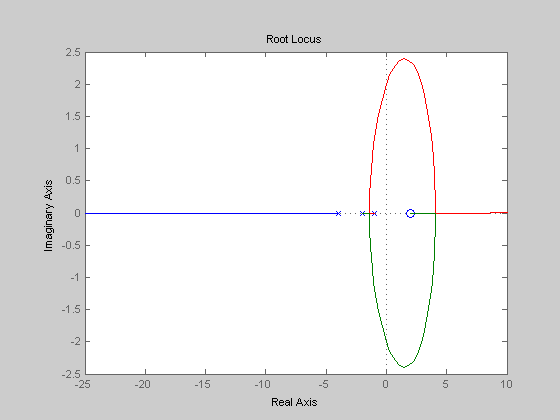
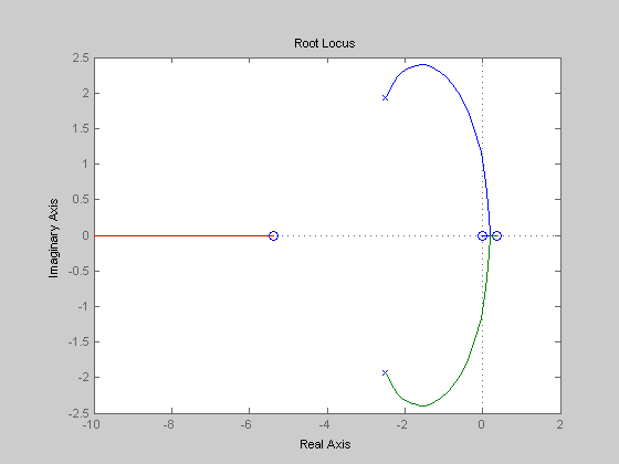
Root locus as T_d varies given K=6 using a 1st order Pade approx.

T = tf([1 5 -2 0], [2 10 20])
rlocus(T);

 
Transfer function:
s^3 + 5 s^2 - 2 s
-----------------
2 s^2 + 10 s + 20
 

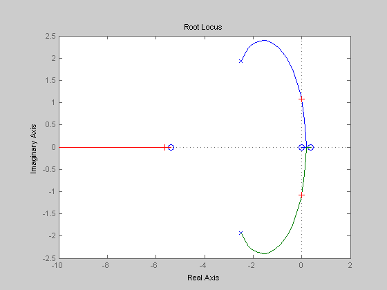
Find a positive T_d for which the system becomes unstable

T_d = rlocfind(T)

Select a point in the graphics window

selected_point =

  -0.0047 + 1.0792i


T_d =

    3.0579

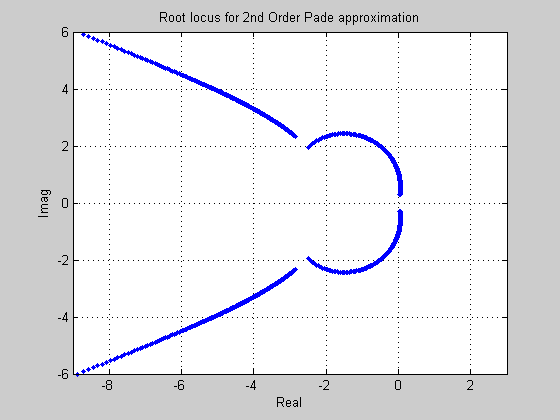
Producing a root locus as T_d varies with a 2nd order Pade Approx.

% setup range of T_d values
Start = 0;
End = 10;
Step = 0.01;

Threshold = 0.002; % threshold for being more or less 0;

% The messy characteristic equation is this:
% pretty(collect(simplify(expand( (s+1)*(s+4)*(Td^2*s^2+6*Td*s+12) + 6*(Td^2*s^2-6*Td*s+12)))))

Tdvec=Start:Step:End;
AllRoots = [];
Tdvals = [];

K = 1;
N = 1;
for I=1:length(Tdvec)
    T_d = Tdvec(I);
    % calculate the roots of the characteristic equation
    % for the current T_d value
    CharEqn = [T_d^2 (6*T_d + 5*T_d^2) (12 + 30*T_d + 10*T_d^2) (60-12*T_d) 120];
    R = roots(CharEqn);
    for J=1:length(R)
            AllRoots(K) = R(J);
            K = K+1;
    end
    % find any roots whose real part is 0 -> on the jw axis
    I = find(real(R)<Threshold  & real(R)>-Threshold);
    if (length(I) > 0)
        Tdvals(N) = T_d;
        N=N+1;
    end

end
plot(real(AllRoots), imag(AllRoots), '.');
axis([-9 3 -6 6]);
grid;
xlabel('Real');
ylabel('Imag');
title('Root locus for 2nd Order Pade approximation');
disp('Created root locus.');

disp('Marginally stable values of T_d');
Tdvals

Created root locus.
Marginally stable values of T_d

Tdvals =

    2.0000    2.0100    2.0200    2.0300    2.0400

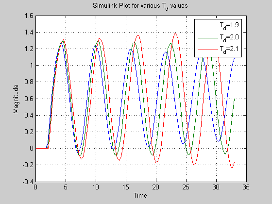
Using SIMULINK to find T_d that causes the system to become unstable

sim_Td=1.9; sim('parte', 33); time1 = simout.time; tdval1 = simout.signals.values;
sim_Td=2.0; sim('parte', 33); time2 = simout.time; tdval2 = simout.signals.values;
sim_Td=2.1; sim('parte', 33); time3 = simout.time; tdval3 = simout.signals.values;

plot(time1, tdval1, time2, tdval2, time3, tdval3);
title('Simulink Plot for various T_d values');
xlabel('Time'); ylabel('Magnitude'); grid;
legend('T_d=1.9', 'T_d=2.0', 'T_d=2.1')

Warning: Using a default value of 0.66 for maximum step size. The simulation step size will be limited to be less than this value.
Warning: Using a default value of 0.66 for maximum step size. The simulation step size will be limited to be less than this value.
Warning: Using a default value of 0.66 for maximum step size. The simulation step size will be limited to be less than this value.

Published with MATLAB® 7.0