Engineering 58 Exam 2 Takehome

Aron Dobos

12 Apr 2005

Problem 4

a) i. Bode plots for 1^st and 2^nd order Pade approximations and ideal time delay. (T_d=1).

>> P1 = tf([-1 2],[1 2])

Transfer function:

-s + 2

------

s + 2

>> P2 = tf([1 -6 12], [ 1 6 12])

Transfer function:

s^2 - 6 s + 12

--------------

s^2 + 6 s + 12

>> Id = tf([1],[1],'inputdelay',1)

Transfer function:

exp(-1*s) * 1

>> bode(P1,P2,Id)

Figure 1. 1^st and 2^nd Order Pade Approx. (T_d=1), Ideal Time Delay

The discrete discontinuities on the magnitude plot are on the order of 10^-15, so it is safe to assume that the magnitude is just 0 dB.

ii. Revised rules for asymptotic bode plots.

Since the ideal time delay does not change the magnitude of the bode plot, the magnitude rule for plotting a Pade approximation is to leave the original magnitude unchanged. Improvised rules for approximate plotting of the phase of the n^th Pade approximation are given.

The following MATLAB program gives the frequency response of 1 to 3 second time delays for each of the first six Pade approximations. The ‘pade’

clear figure;

hold on;

for td=1:3

for n=1:6

[num den] = pade(td, n);

disp(sprintf('Order %d Pade approximation (Td=%d)\n', n, td));

T = tf(num,den)

roots(num)

roots(den)

bode(T)

end

end

hold off;

Figure 2. Phase of 1à6 Order Pade Approx. with T_d= 1à3 s

From this graph, we can see that the low frequency asymptote increases by 360 degrees for each increase of two orders of the Pade approximation. The high frequency asymptote is always 180 degrees or 0 degrees, depending on whether the order of the approximation is even or odd. An increase in the time delay shifts the phase to the left. Looking at the 1^st order approximation shown in Figure 1 for T_d=1, the center frequency w₀ seems to be at 2 rad/sec, which would make sense given the original Bode plot rules, if the 1^st order Pade approximation transfer function is written in the appropriate form given below:

Therefore it is assumed for lack of better insight that the center frequency, the approximate inflection point of the Pade phase curve, is used to plot the asymptotic phase approximation for the Pade approximation is this w₀.

The 3^rd order Pade approximation (T_d=1) is

The roots of the numerator are the negative of the denominator roots, and are given below.

3.6778 + 3.5088i

3.6778 - 3.5088i

4.6444

The denominator polynomial can be written as

For the 2^nd order complex pole the natural frequency and damping ratio are

Using the asymptotic phase equations for a standard 2^nd order pole, we plot a line from the low frequency asymptote to the high frequency asymptote starting at

rad/sec

to

rad/sec.

Looking at the phase plot for the actual 3^rd order Pade approximation, these frequencies appear appropriate for the starting and ending points of the connecting line. The frequency of the real root at s=4.6444 is about at the center of the curve.

The phase plot of the 3^rd order Pade approximation is given below.

Figure 3. P₃(s) Phase diagram.

The denominator of n^th order Pade approximation for n > 2 and n is odd can always be written factored into the form

since there is always a real pole. The zeros of the numerator are the negated zeros of denominator polynomial. From the discussion of the 3^rd order approximation, we decided to use the value of the real pole as the ‘center’ frequency of the inflection point. For lack of a better idea, this is the frequency we will use.

For an even order Pade approximation, simply choose one of the natural frequencies I suppose.

In summary, the updated asymptotic bode plot rules for an n^th order Pade approximation are:

	Magnitude	Phase
Pade(n, Td)	0 dB	1. Low frequency asymptote at 2. High frequency asymptote at 3. Connect from to if a 2^nd order underdamped pole, otherwise use from 0.1w to 10w for a real root.

We can also write the rules so that the phase always starts at 0 degrees, since adding 360 does not change the actual response. In this case the Bode plot rules are given by:

	Magnitude	Phase
Pade(n, Td)	0 dB	1. Low frequency asymptote at 2. High frequency asymptote at 3. Connect from to if a 2^nd order underdamped pole, otherwise use from 0.1w to 10w for a real root.

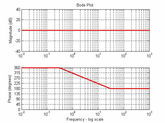iii. Using these rules from the first table, the Bode plot for the 1^st order Pade approximation is shown below.

Figure 4. Asymptotic Plot of 1^st Order Pade Approx. (T_d=1)

This plot compares reasonably favorably with the MATLAB generated phase plot for the 1^st order Pade approximation.

b) Determine the time delay to make the system marginally stable using Nyquist or Bode plot. The uncompensated system is shown below.

Figure 5. Uncompensated system margins.

>> Gp = tf([6],poly([-1 -4]))

Transfer function:

6

-------------

s^2 + 5 s + 4

>> margin(Gp)

i. For the 1^st Order Pade Approx.

To find the time delay required to make the system marginally stable, we iterate through time delays, and stop as soon as the closed loop transfer function has roots on the jw axis. The MATLAB code to do this for the first order Pade approximation is given below.

function [Td, Wn] = pade1unstable(start, granularity, final)

Gp = tf([6],poly([-1 -4]));

for Td = start:granularity:final

T = feedback(Gp*tf([-Td 2],[Td 2]),1);

[num, den] = tfdata(T, 'v');

rden = roots(den);

R = find(real(rden) > 0);

if (length(R)>0)

Wn = imag(rden(R(1)));

return;

end

end

Guessing that the required time delay was approximately 1.5 seconds or more, the function is called with a Td step size of 0.0001. The natural frequency of the oscillation is returned also.

>> [T w] = pade1unstable(3.2,.00001,3.3)

T =

3.2209

w =

1.0510

ii. For the 2^nd Order Pade Approx.

We use the same methodology for the 2^nd order approximation. The MATLAB code is given below.

function [Td, Wn] = pade2unstable(start, granularity, final)

Gp = tf([6],poly([-1 -4]));

for Td = start:granularity:final

T = feedback(Gp*tf([Td^2 -6*Td 12],[Td^2 6*Td 12]),1);

[num, den] = tfdata(T, 'v');

rden = roots(den);

R = find(real(rden) > 0);

if (length(R)>0)

Wn = imag(rden(R(1)));

return;

end

end

>> [T w]=pade2unstable(2, 0.00001, 2.2)

T =

2.0159

w =

1.0510

Note that the oscillation frequency for the marginally stable case is the same as with the 1^st order Pade approximation. This makes sense since the magnitude is unchanged, only the phase, so the crossover frequency does not change.

iii. For the ideal time delay.

The phase of an ideal time delay is . Since the phase margin is 119 degrees, we wish to decrease the phase by 119 degrees at the crossover frequency so that the system gain is 1 with -180 degrees phase angle. The ideal delay does not affect the magnitude, so the crossover frequency does not change, and is 1.05 radians (read from the bode plot).

Solving the equation , we get .

c) Oscillation frequencies for the marginally stable systems.

The oscillation frequency for each of the systems is at the crossover frequency because neither the Pade approximations nor the ideal delay change the magnitude plot. Therefore, the systems will oscillate at 1.05 rad/sec. The frequency in Hertz is therefore . The period is thus 5.984 s. The step response of each of the marginally stable delayed systems are shown below, and thus the oscillation frequency stands verified, as the period is clearly about 6 seconds.

1^st and 2^nd Order Pade Approximations:

Ideal time delay case:

d)

i. Bode and Nyquist plots for system .

ii.

This system is necessarily unstable because the time delay decreases phase, and the original transfer function was already marginally stable with a constant -180 degrees phase.

iii. A PD controller increases phase, and therefore can potentially stabilize the system. The same is true for the lead controller. It might be difficult to find a controller to stabilize the time delayed system because the phase drops off so quickly. The system without the time delay should be very straightforward to control with a PD or lead controller.