Engineering 6 Lab 1:
Concurrent Force Equilibrium in 3-D
Paul Agyiri, Aron Dobos
13 February 2005
Abstract
In this lab, the weight of a mass hanging in equilibrium from three cords was determined, as well as the friction coefficients of the three pulleys involved. From the collective class data, the average weight was determined to be 1077 grams, with an error of approximately ± 2.5%. The average friction coefficients for the pulleys 1, 2, and 3 were determined to be 0.208, 0.131, and 0.158, with standard deviations of 0.008, 0.004, and 0.003, respectively. The efficiencies of the three pulleys were calculated to be 96%, 97.5%, and 96.7%, respectively.
Procedure
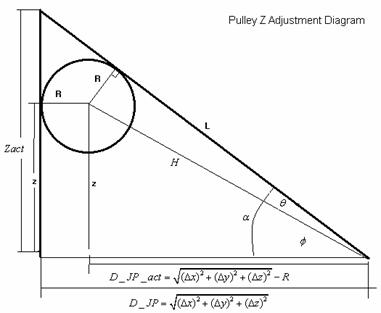
Three pulleys were set up as shown in the sketch of the apparatus with an unknown weight being supported at the point where the three ropes that hung from each pulley met. This setup was done above a floor with and x-y grid on it. The values of three specific weights were recorded and these weights were hung on the pulleys, with one weight hanging from each pulley. The unknown weight was pulled down and slowly allowed to reach equilibrium position from the bottom (that is slowly allowed to come to rest). The x, y and z positions of the unknown weight were measured and recorded. Using the same set of weights, the unknown weight was raised up slightly and slowly guided downwards until it came to equilibrium again. The new x, y and z coordinates were measured and recorded. A diagram of the pulley-weight configuration is shown below in Figure 1.
Figure 1. Setup

Free Body Analysis
The displacement vectors from the junction coordinate to each of the three pulleys is calculated by subtracting the respective X, Y, and Z components of the junction from the pulley coordinates. The Z coordinate was adjusted to account for the radius of the pulley.
The first step in the free body analysis is to adjust for the actual Z coordinate using the known radius of the pulley. The actual distance from the junction to the pulley sheave in the X-Y plane is calculated using the equation below.
![]()
Given this distance, the angle phi can be calculated with the Pythagorean Theorem, as well as the hypotenuse H of the smaller right triangle. With H and R, the angles theta and alpha are determined to be
![]() ,
,
and Zact is given by
![]() .
.
To calculate the weight of the hanging object, it is assumed that the pulleys are frictionless and thus the weight at the end of each cord is equal to the tension in that cord. Given the adjusted three dimensional displacement vectors, the Z component of each cord tension can directly be determined by multiplying the cord tension by the normalized Z component vector. Summing the Z components of each of the three tensions gives the weight of the hanging objects, since the sum of the forces in the Z direction must be zero:
![]()
where ![]() is the normalized ith displacement
vector in the z direction.
is the normalized ith displacement
vector in the z direction.
An estimate for the actual weight is determined by averaging the weight from the ‘above’ run with the weight obtained from the below run.
![]()
Given the average mass, the friction can be calculated for approaching equilibrium from above and below.
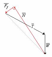
Diagram For Calculating Friction Force
Taking the difference between AverageMass and MassAbove (or MassBelow) gives the difference in the Z-component of the tension between the actual and friction-less tension. The actual tension is thus given by
![]()
The friction force is determined by summing torques around the pulley center.
![]()
The normal force vector to the friction force from the weight junction is readily obtained by the Pythagorean Theorem.
![]()
The coefficient of friction and the pulley efficiency are given by the following relationships below.
![]()
Results
The data and results obtained for each ‘above’ and ‘below’ run is included below in Table 1. The results were calculated automatically by the runall.m and calcforces.m MATLAB scripts.
Table 1. Collective Class Weight, Above/Below XYZ
Data with Calculated Results for each run.
|
Run |
Wt 1 |
Wt 2 |
Wt 3 |
AX |
AY |
AZ |
BX |
BY |
BZ |
Mass |
P1 Mu |
P2 Mu |
P2 Mu |
|
1 |
683 |
748 |
729 |
-1 |
38.3 |
78.4 |
-1.9 |
39.5 |
75 |
1070.02 |
0.1193 |
0.0869 |
0.1177 |
|
2 |
894 |
948 |
488 |
-16 |
4.2 |
79.8 |
-17.1 |
4.8 |
77.4 |
1162.04 |
0.091 |
0.0461 |
0.1433 |
|
3 |
604 |
552 |
785 |
5.6 |
29.4 |
77.2 |
3.5 |
30.6 |
72.2 |
1052.51 |
0.1671 |
0.1398 |
0.1453 |
|
4 |
763 |
749 |
995 |
7.5 |
26.8 |
88.5 |
6.1 |
27.9 |
86.6 |
1075.29 |
0.0612 |
0.0452 |
0.0573 |
|
5 |
328 |
878 |
655 |
7.5 |
78 |
65.8 |
7 |
77 |
60.2 |
1098.33 |
0.2813 |
0.1239 |
0.1491 |
|
6 |
432 |
692 |
787 |
12.2 |
41 |
72 |
10.2 |
44.6 |
67.6 |
1065.79 |
0.1587 |
0.0886 |
0.1021 |
|
7 |
627 |
512 |
550 |
-7.4 |
34.6 |
64.1 |
-8.9 |
35.5 |
57.4 |
1054.49 |
0.1845 |
0.1775 |
0.2074 |
|
8 |
456 |
693 |
814 |
12 |
39.1 |
74.8 |
10.5 |
40.5 |
70.1 |
1066.08 |
0.1921 |
0.1091 |
0.1274 |
|
9 |
379 |
308 |
875 |
24.6 |
12.5 |
76 |
21.5 |
15.8 |
67.6 |
1059.44 |
0.1847 |
0.1733 |
0.1119 |
|
10 |
379 |
705 |
494 |
2.1 |
69.4 |
49.4 |
0.8 |
70 |
40.3 |
1081.26 |
0.3005 |
0.1694 |
0.2357 |
|
11 |
503 |
576 |
624 |
1.6 |
41.1 |
61.5 |
0.8 |
41.8 |
55.8 |
1066.87 |
0.1817 |
0.1367 |
0.1545 |
|
12 |
433 |
482 |
567 |
3.1 |
40.8 |
48 |
1.4 |
41.4 |
34.8 |
1064.36 |
0.3506 |
0.2748 |
0.275 |
|
13 |
324 |
848 |
416 |
0.6 |
96.6 |
56.5 |
0.1 |
94.8 |
46.6 |
1096.19 |
0.3077 |
0.1518 |
0.2428 |
|
14 |
324 |
744 |
867 |
18.3 |
43.5 |
76.3 |
16.8 |
46.4 |
68.6 |
1052.91 |
0.4456 |
0.1687 |
0.1945 |
|
15 |
703 |
903 |
596 |
-6.3 |
57.4 |
75.4 |
-7.5 |
58.3 |
72.6 |
1090.55 |
0.0955 |
0.0707 |
0.1118 |
Table 2. Summary of Pulley Friction Coefficients, Standard
Deviations, and Efficiencies.
|
Pulley |
Mu |
StdDev |
Efficiency
(%) |
|
1 |
0.2081 |
0.008 |
96.05 |
|
2 |
0.1308 |
0.0043 |
97.54 |
|
3 |
0.1584 |
0.0033 |
96.77 |
Table 3. Final Mass and Error Estimates
|
Object Mass |
Approx. Error |
|
1077.1 |
~ 4 - 6% |
Error Considerations
We can calculate the approximate error in the weight of the hanging mass by considering the difference between the weight obtained from ‘below’ runs and ‘above’ runs, and comparing them to the average weight. This gives an estimate of the spread of the weight values obtained, and clearly includes the uncertainties resulting from the friction in the pulleys.
Error in the weight due to friction =
(weight from below – weight from above)/2
average weight
(1128.4 –
1078.7)/2
(1128.4 + 1078.7)/2
= 2.25%
Another approximate measure of the error can be obtained from the sum of forces in the X and Y directions. Ideally, these forces should sum to 0, since the hanging mass is in equilibrium. Taking the root mean square (RMS) of the X and Y tension sums gives an estimate of the total XY error, and dividing this error value by the Z tension results in a value that represents the total error in the measurement of the Z tension. Averaging all of these error values together gives an error of approximately 7 % from all the ‘above’ and ‘below’ runs. This error is much greater than the error estimate obtained from the much simpler calculation described above. A possible reason is that in this case, the error in each individual force equilibrium calculation is a greater percentage, whereas when all of the ‘above’ and ‘below’ runs are averaged, the result evens out and represents a smaller spread of values, even though the actual error invovled in calculating the final averages might have been greater.
If the total spread of the ‘above’ and ‘below’ runs is considered instead of just the difference between the mean weight value, the basic error calculation gives 2*2.25 = 4.5 % error, which seems more reasonable next to the XY error calculation. Given these various methods of calculating error, it is probably safe to conclude that the final error in the weight of the hanging mass is approximately between 4 and 6 percent.
Discussion
The frictional forces in the pulleys produced a difference in the unknown weight which was calculated to be a percentage error of approximately 4-6%. This is a relatively small error, and as a result it is probably safe to assume for most applications that the pulley is indeed frictionless. If more precision is required in obtaining weight values of hanging masses, the friction in the pulleys probably should not be neglected. Knowing how the friction affects tests reaching equilibrium from above and from below, it should be enough to do both tests and average the values, as the frictional effects should cancel out and give an accurate value for the weight of the hanging mass.
MATLAB CODE
runall.m
% runall.m
% Aron
Dobos, Spring 2006
%
% Calculates all the masses, pulley frictions, and average XY
errors,
% and
averages them. The variable AllData must be in the workspace.
% It is just a big table contain all the data points in the
following
%
format. The table can have
as many rows as needed.
%
% [
Weights ] [ FromAboveXYZ
] [ FromBelowXYZ
]
%
% 763
749 995 7.5
26.8 88.5 6.1
27.9 86.6
% 328
878 655 7.5
78 65.8 7
77 60.2
% 432
692 787 12.2
41 72 10.2
44.6 67.6
% 627
512 550 -7.4
34.6 64.1 -8.9
35.5 57.4
% 456
693 814 12
39.1 74.8 10.5
40.5 70.1
% 379
308 875 24.6
12.5 76 21.5
15.8 67.6
%
[M N] = size(AllData);
fp = fopen('mresults.txt', 'w');
Weights = zeros(M, 3);
Above = zeros(M, 3);
Below = zeros(M, 3);
XYError = 0;
AllMus = zeros(M, 3);
AvgMus = zeros(3, 1);
AvgEff = zeros(3, 1);
MuStdDev = zeros(3,1);
AverageMass = 0;
AvgFrictionForce = 0;
for I=1:M
Weights(I,:) = AllData(I, 1:3) / 1000;
% weights in kilograms
Above(I,:) = AllData(I, 4:6) / 39.3700787; %
locations in meters
Below(I,:) = AllData(I, 7:9) / 39.3700787; %
locations in meters
% calculate all values for the I-th run using the calcforces
function
calcs
= calcforces(Weights(I,:), Above(I,:), Below(I,:));
for K=1:3
AllMus(M,K) = calcs.PulleyMuAvg(K);
AvgMus(K) = AvgMus(K) + calcs.PulleyMuAvg(K);
AvgEff(K) = AvgEff(K) + calcs.PulleyEffAvg(K);
end
% average the friction forces
AvgFrictionForce
= AvgFrictionForce + calcs.AvgFriction;
% average the masses
AverageMass = AverageMass + calcs.ActualMass;
% average the RMS errors from 0,0 for the XY coordinate tensions
XYError = XYError + calcs.AvgErrXY;
fprintf(fp, '%d\t%d\t%d\t', Weights(I,1), Weights(I,2), Weights(I,3));
fprintf(fp, '%.1f\t%.1f\t%.1f\t', Above(I,1),
Above(I,2), Above(I,3));
fprintf(fp, '%.1f\t%.1f\t%.1f\t', Below(I,1),
Below(I,2), Below(I,3));
fprintf(fp, '%.2f\t%.4f\t%.4f\t%.4f\n', calcs.ActualMass, calcs.PulleyMuAvg(1),
calcs.PulleyMuAvg(2), calcs.PulleyMuAvg(3));
end
AvgFrictionForce = AvgFrictionForce
/ M;
AverageMass = AverageMass / M;
XYError = XYError / M;
% average
all the frictions and efficiencies for each pulley
for K=1:3,
AvgMus(K) = AvgMus(K) / M;
AvgEff(K) = AvgEff(K) / M;
end
%
calculate the standard deviations for the pulley frictions
for K=1:3
fsum
= 0;
for I=1:M
fsum
= ( AllMus(M,K) - AvgMus(K)
)^2;
end
MuStdDev(K) = sqrt(fsum)
/ (M-1);
end
fclose(fp);
% display the results.
AverageMass
XYError
AvgMus
MuStdDev
AvgEff
AvgFrictionForce
calcforces.m
function [ret] = calcforces(hanging_weights, above_data, below_data)
%%%%%%%%%%%%%%%%%%%%%%%%%%%%%%%%%%%%%%%%%%%%%%%%%%%%%%%%%%%%%%%%%%%%%%%%
% calcforces.m
% Matlab script to calculate tensions, weights, and frictions
% Units are inches, grams
% Aron
Dobos, Spring 2005
%
% PFromAbove = [7.5 78 65.8];
% PFromBelow = [7 77 60.2];
%
% usage: calcforces(hanging_weights[1x3], above_data[1x3],
below_data[1x3])
%
% Example:
% > PFromAbove = [7.5 78 65.8];
% > PFromBelow = [7 77 60.2];
% >
Weights = [328 878 655];
% > calcforces(Weights,
PFromAbove, PFromBelow);
% ABOVE:
tension 1: Alpha=28.374703 degrees, Z=120.704820
% ABOVE:
tension 2: Alpha=40.355489 degrees, Z=120.968397
% ABOVE:
tension 3: Alpha=32.473082 degrees, Z=120.778002
% Mass for
run ABOVE=1091.953522 grams
% BELOW:
tension 1: Alpha=31.051536 degrees, Z=120.750897
% BELOW:
tension 2: Alpha=42.729991 degrees, Z=121.042040
% BELOW:
tension 3: Alpha=35.270283 degrees, Z=120.837251
% Mass for
run BELOW=1161.211849 grams
% ABOVE
Pulley 1 Mu=0.269096
% ABOVE
Pulley 2 Mu=0.122617
% ABOVE
Pulley 3 Mu=0.145532
% BELOW
Pulley 1 Mu=0.286309
% BELOW
Pulley 2 Mu=0.126376
% BELOW
Pulley 3 Mu=0.152947
%
% ans =
%
% AverageMass:
1.1266e+003
% PulleyMuAvg:
[0.2777 0.1245 0.1492]
% data: [1x2 struct]
%
%%%%%%%%%%%%%%%%%%%%%%%%%%%%%%%%%%%%%%%%%%%%%%%%%%%%%%%%%%%%%%%%%%%%%%%%
Weights = hanging_weights;
data(1).Junction = above_data;
data(1).RunName = 'ABOVE';
data(2).Junction = below_data;
data(2).RunName = 'BELOW';
% Define
the known data points
SnapWeight = 9 / 1000; % in kilograms
JunctionSnapWeight = 13 / 1000; % in
kilograms
% pulley
locations in meters
P1 = [-60 0 119]
/ 39.3700787;
P2 = [0 144 119]
/ 39.3700787;
P3 = [48 0 119]
/ 39.3700787;
PRadius = 1.5 / 39.3700787; % pulley radius
AxleRadius = 0.1875 / 39.3700787; % axle
radius
Pullies = [ P1; P2; P3 ];
Weights =
Weights + SnapWeight; % add the snap weight
% get the forces (frictionless cable tensions) in newtons
WeightForces = Weights * 9.81;
ret.AverageMass = 0;
ret.AvgErrXY = 0;
% iterate
through the 'above' run and the 'below' run
for D=1:2
% initialize
some variables for the data set.
data(D).Displace =
zeros(3,3);
data(D).Normalized
= zeros(3, 3);
data(D).D_JP =
zeros(3,1);
data(D).H =
zeros(3,1);
data(D).Zact = zeros(3,1);
data(D).D_JP_act = zeros(3,1);
data(D).Alpha =
zeros(3,1);
data(D).Phi =
zeros(3,1);
data(D).Theta =
zeros(3,1);
for I=1:3
% calculate the displacement
vectors for this run
data(D).Displace(I,:)
= Pullies(I,:) - data(D).Junction;
% calculate the distance from the
junction to the pulley
data(D).D_JP(I) = sqrt(
data(D).Displace(I,1)^2 + data(D).Displace(I,2)^2 );
% adjust the distance to get the
actual distance from the junction
% to the center of the pulley
sheave
data(D).D_JP_act(I) = data(D).D_JP(I) - PRadius;
% calculate the hypotenuse of the the triangle whose base is the
% distance from J to the pulley
sheave and height is the delta Z.
data(D).H(I) = sqrt(
data(D).D_JP_act(I)^2 + data(D).Displace(I,3)^2 );
% calculate the Phi angle in the
triangle (See drawing)
data(D).Phi(I)
= atan2(data(D).Displace(I,3), data(D).D_JP_act(I)) *
180/pi;
% likewise calculate theta for the
smaller triangle
data(D).Theta(I)
= asin( PRadius /
data(D).H(I) ) * 180/pi;
% determine alpha which is the
actual angle the cord makes with the
% horizontal axis
data(D).Alpha(I)
= data(D).Phi(I) + data(D).Theta(I);
% from alpha calculate the actual
Z
data(D).Zact(I) = data(D).D_JP_act(I)*tan(data(D).Alpha(I)*pi/180);
disp( sprintf('%s: tension %d: Alpha=%f degrees, Z=%f', data(D).RunName, I, data(D).Alpha(I), data(D).Zact(I)+data(D).Junction(3)));
% update the displacement vector
with the actual Z coordinate
data(D).Displace(I,3)
= data(D).Zact(I);
% normalize to obtain unit vectors
for the displacements
data(D).Normalized(I,:) =
data(D).Displace(I,:) / norm(data(D).Displace(I,:));
end
data(D).TSumX = 0;
data(D).TSumY = 0;
data(D).TSumZ = 0;
% sum the force components in the X Y and Z directions
assuming no
%
friction.
for I=1:3
data(D).TSumX = data(D).TSumX + WeightForces(I)*data(D).Normalized(I,1);
data(D).TSumY = data(D).TSumY + WeightForces(I)*data(D).Normalized(I,2);
data(D).TSumZ = data(D).TSumZ + WeightForces(I)*data(D).Normalized(I,3);
end
% take
the RMS (root-mean-square) of the X and Y sums (which should be
% zero) to get an estimate of the
error
data(D).ErrXY = sqrt(data(D).TSumX^2 +
data(D).TSumY^2);
% now take obtain the percentage
error from the Z sum to get an idea of
% how off the Z sum could be
data(D).ErrXYPercentOfZ = data(D).ErrXY /
data(D).TSumZ * 100;
disp(sprintf('XYZ sums: %f %f %f (RMS %f err %f)', data(D).TSumX, data(D).TSumY, data(D).TSumZ, data(D).ErrXY, data(D).ErrXYPercentOfZ));
ret.AvgErrXY = ret.AvgErrXY + data(D).ErrXYPercentOfZ;
% the mass is just the sum of the
Z components of the tensions
% divided by gravitational
acceleration
data(D).Mass =
data(D).TSumZ / 9.81;
ret.AverageMass =
ret.AverageMass + data(D).Mass;
disp(sprintf('Mass for run
%s=%f grams', data(D).RunName, data(D).TSumZ));
end
%
determine the average mass
ret.AverageMass = ret.AverageMass
/ 2;
ret.AvgErrXY = ret.AvgErrXY
/ 2;
% now
calculate all the pulley frictions from both above and below runs
for D=1:2
% initialize
the friction variables
data(D).Frictions
= zeros(3,1);
data(D).Normals = zeros(3,1);
data(D).PulleyMu = zeros(3,1);
data(D).Tensions =
zeros(3,1);
data(D).Efficiency
= zeros(3,1);
data(D).MassDiff = abs(data(D).Mass - ret.AverageMass);
for I=1:3
% calculate the actual tension in
the cord by using the mass
% difference from the run and the
average
data(D).Tensions(I)
= WeightForces(I) - 9.81*data(D).MassDiff
* data(D).Normalized(I,3);
% determine the friction force by
summing torques around the pulley
% wheel, accounting for the sheave
radius and outer radius
data(D).Frictions(I)
= 9.81*data(D).MassDiff * data(D).Normalized(I,3) * PRadius / AxleRadius;
% calculate the magnitude of the
sheave normal vector by
% the pythagorean theorem
data(D).Normals(I)
= sqrt( (data(D).Tensions(I)*data(D).Normalized(I,3)
+ WeightForces(I))^2 - data(D).Frictions(I)^2);
% determine Mu
= mag(F)
/ mag(N)
data(D).PulleyMu(I) = data(D).Frictions(I) / data(D).Normals(I);
% determine the efficiency of each
pulley
data(D).Efficiency(I) = 1 - data(D).MassDiff*9.81 * data(D).Normalized(I,3) / ((WeightForces(I)+data(D).Tensions(I))/2);
disp(sprintf('%s Pulley %d Mu=%f Eff=%f Friction=%f', data(D).RunName,
I, data(D).PulleyMu(I), data(D).Efficiency(I),
data(D).Frictions(I) ));
end
end
% average
the mu values for each pulley resulting from the
% above
and below runs
ret.AvgFriction = 0;
for I=1:3
ret.PulleyMuAvg(I) = 0;
ret.PulleyEffAvg(I) = 0;
for D=1:2
ret.PulleyMuAvg(I) = ret.PulleyMuAvg(I) +
data(D).PulleyMu(I);
ret.PulleyEffAvg(I) = ret.PulleyEffAvg(I) +
data(D).Efficiency(I);
ret.AvgFriction
= ret.AvgFriction + data(D).Frictions(I);
end
ret.PulleyMuAvg(I) = ret.PulleyMuAvg(I) / 2;
ret.PulleyEffAvg(I) = ret.PulleyEffAvg(I) / 2;
end
ret.AvgFriction = ret.AvgFriction
/ 6;
% subtract
the known snap weight from the averaged mass
ret.ActualMass = ret.AverageMass
- JunctionSnapWeight;
% return all calculated data values
ret.data = data;