Engineering 6 Tensile Test Report
21 March 2005
Fortman-Roe, Agyiri, Benn, Dobos
Abstract (Dobos)
In this lab, standard .505 2024-aluminum and HDPE specimens were destructively tested using a computer controlled, mechanically driver Universal Testing Machine. The resulting stress-strain curves obtained from the testing machine were analyzed using MATLAB to obtain various specimen parameters including the Modulus of Elasticity (E), 0.2% Yield Strength, Ultimate Tensile Strength, Percent Elongation at Rupture, Modulus of Resilience, and the Modulus of Rupture (Toughness). A first order numerical integration routine was also developed in MATLAB code to assist the analysis procedures.
Introduction (Fortmann-Roe,
Agyiri, and Benn)
To conduct this experiment we needed two tensile test specimens. The first specimen was a 2024 Aluminum bar with a diameter of .5 inches and a height of 2 inches. The second specimen we used was a High-Density Polyethylene (HDPE) bar with similar dimensions to the aluminum sample.
We placed these specimens into a Universal Testing Machine
(UTM) housed in the basement of Papazian. This
machine, manufactured in
We hooked the UTM and DMT up to computer so that their measurements could be recorded in real-time as testing proceeded. The software we used to handle and monitor this recording process was Mtest.
Once everything had been setup and configured we proceeded with the tests themselves! The first specimen tested was the HDPE sample. When tested, this material exhibited a number of rather interesting qualities and features. As it was increasingly stressed, the HDPE displayed significant necking. This necking originated at the middle of the specimen and gradually spread outwards from there. The necking was rather interesting for at the location of necking the material would shrink in diameter and elongate. As it shrunk, the sample lost the semi-translucent shimmer it had originally possessed and became a hard white. This process is called linearization and results in the material becoming extremely tough (it is the process employed in the creation of Kevlar). Furthermore, as the HDPE was increasing linearized we observed the phenomenon that the diameter at the top of the necking was smaller than that at the bottom. We believe that this is due to the heat generated during the process and its upwards movement.
Sketches of the distinct failure modes of the two specimens are shown below in Figure 0.
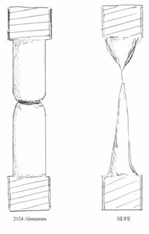
Figure 0. Sketches of Failure Modes for 2024 Aluminum and HDPE Specimens
After we had stressed the HDPE for a significant period of time (so that it was now 7.5 times its original length and had been completely linearized) we experienced a fracture at the top of the specimen. When examined afterwards, the fracture looked like the fraying of a rope with individual strands and segments. At this point, a section that had been completely linearized displayed an 86% reduction in area.
The second specimen was the 2024 Aluminum bar. There was a significant difference in the behavior of this material when compared to that of the HDPE. Firstly, there was less dramatic necking throughout the length of the bar except at the point of fracture which had a slightly more significant necking than the rest of the length of the bar. The surface of fracture, which was in the middle of the length of the bar of this material was jagged, which is different from what was observed in the HDPE, which was more tapered. During fracture, there was a large gunshot sound which is in contrast to the silent fracture of the HDPE. The strain obtained was 16.5% and the narrowest diameter of the 2024 Aluminum just before the point of rupture was 0.455in which is only a 0.1in change in diameter, a significantly less change in diameter when compared to that of the HDPE.
Analysis Procedures
(Dobos)
The procedures followed for parameter determination for the aluminum specimen are outlined below.
Modulus of Elasticity: From the stress-strain curve, two points were chosen that appeared to be in the linear region of the graph. From these two points, the linear slope was calculated, which in fact is E. The points chosen for this calculation are shown in Figure 1 for the aluminum specimen.
E2024
= (4.321*10^4 - 1.514*10^4) / ( 0.0034 - 0.0009) = 11228000 psi;
A more accurate method of determining the modulus of elasticity would be to make linear fit to the linear region of the data to obtain the slope. Another way would be to write a loop that calculates the 1st order derivatives of the stress vs. strain, and returns the maximum derivative found in the linear region. These methods were not pursued due to time constraints, and the two-point method seemed reasonable given how linear the slope was in the elastic region for the aluminum.
0.2% Yield Strength: Having calculated E, the equation of a line parallel to the linear region but passing through 0.002 in/in strain was calculated. The equation of this line is y = Ex - 0.002E, and is plotted on the stress strain diagram in Figure 1. The intersection of this line and the experimental stress-strain curve gives the 0.2% yield strength which is clearly annotated on the diagram.
Ultimate Yield Strength: The maximum value of the stress at the point of rupture was used to obtain this parameter by inspection of the graph.
Modulus of Resilience: The stress-strain data was sectioned at the elastic limit, and the first part was integrated over the strain to obtain this parameter, as described in the professor’s laboratory handout.
Modulus of Rupture: The stress was integrated from zero strain to the strain at rupture.
Elongation at Rupture: The elongation was obtained by extending a line with slope E from the point of rupture. The intersection of this line and 0 gives the strain at failure. Multiplying by the initial length (2”) gives the elongation at failure.
Reduction in Area: The ratio of the final area to the initial area gives the percent of area remaining at rupture. The reduction of area is therefore 1 minus this value.
The same methods were applied to determine the parameters for the HDPE specimen, except that the Modulus of Rupture could not be calculated since the logged data did not extend to the point of rupture.
Results (Dobos)
The parameters are summarized below for the two specimens in Table 1.
|
Parameter |
A2024 |
HDPE |
Units |
|
Modulus
of Elasticity |
11228 |
114 |
ksi |
|
0.2%
Yield Strength |
51420 |
2273 |
psi |
|
Ultimate
Yield Strength |
69580 |
3867 |
psi |
|
Modulus
of Resilience |
122.79 |
28.37 |
psi |
|
Modulus
of Rupture |
11338 |
n/a |
psi |
|
Elongation
at Rupture |
0.34142 |
15 |
inches |
|
Reduction
of Area |
18.4 |
88.8 |
% |
Table 1. Experimentally Determined Parameter Values
An annotated stress-strain curve is given in Figure 1 for the aluminum specimen.
Figure 1. Stress-Strain Characteristics for 2024 Aluminum
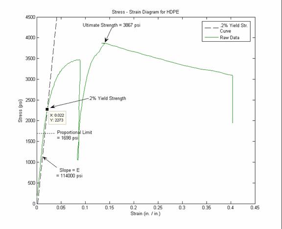
Figure 2. Stress-Strain Characteristic for HDPE Specimen
Discussion (Dobos)
The specimen parameters were successfully determined using the methods described above. The testing machine did not provide reasonable values for aluminum due to a glitch, so we cannot provide any comparisons. For the HDPE sample however, the values compare favorably as seen below in Table 2.
|
Parameter |
Calculated |
Machine |
Units |
|
Modulus
of Elasticity |
114000 |
94263 |
psi |
|
0.2%
Yield Strength |
2273 |
2625 |
psi |
|
Reduction
of Area |
88.8 |
89.11 |
% |
Table 2. Comparison of Calculated HDPE Parameters to Machine-determined values.
The discrepancies can easily be accounted for in the approximate methods used to determine the calculated values. Also, the strain gauge slipped slightly on the smooth nylon surface, thereby introducing potentially significant errors in the measurement of the strain data. Despite such error, the values are reasonably close.
Acknowledgements (Dobos)
Professor Orthlieb is thanked for operating the Universal Testing Machine and putting himself between the rupturing specimens and the students.
Tau Beta Pi is thanked for holding a MATLAB workshop.
Appendices
MATLAB Code
do2024.m
%% Create 2024 Stress Strain Diagram
% Aron Dobos 2005 E6 Tensile Test Lab
load
alldata.mat
% these values are taken from the
cursors on the plot
E2024 = (4.321*10^4 - 1.514*10^4) / ( 0.0034 - 0.0009);
x1
= strain_2024;
y1 = force_2024 / area_2024;
x2
= 0.002:0.0005:0.007;
y2 = E2024*line_x-.002*E2024;
x3
= 0.1707:0.0001:0.1769;
y3 = E2024*line_x-1916653.2;
% calculate modulus of resilience
mresX
= strain_2024(1:290);
mresY
= force_2024(1:290)/area_2024;
ModulusResilience2024 = myint(mresX, mresY);
% calculate modulus of rupture
ModulusRupture2024 = myint(strain_2024,
force_2024/area_2024);
%CREATEFIGURE(X1,Y1,X2,Y2,X3,Y3)
% X1: vector of x data
% Y1: vector of y data
% X2: vector of x data
% Y2: vector of y data
% X3: vector of x data
% Y3: vector of y data
% Auto-generated
by MATLAB on 21-Mar-2005 14:08:41
%% Create figure
figure1 = figure('FileName','\\130.58.237.132\uploads\e6\tensile\2024_E_calc.fig');
%% Create axes
axes1 = axes('Parent',figure1);
title(axes1,'Stress-Strain
Diagram for 2024 Aluminum Specimen');
xlabel(axes1,'Strain (in/in)');
ylabel(axes1,'Stress (psi)');
grid(axes1,'on');
hold(axes1,'all');
%% Create plot
plot1 = plot(...
x1,y1,...
'Parent',axes1,...
'DisplayName','Experimental Data');
%% Create plot
plot2 = plot(...
x2,y2,...
'Parent',axes1,...
'DisplayName','0.2% Yield Strength Line');
%% Create text
text1 = text(...
'BackgroundColor',[1 1 1],...
'FontWeight','bold',...
'Position',[0.008 3.368e+004 0],...
'String','\leftarrow Slope = E = 1.1228e+7',...
'Parent',axes1);
%% Create text
text2 = text(...
'FontWeight','bold',...
'Position',[0.01065 5.127e+004 36.64],...
'String','\leftarrow 0.2% Yield Strength',...
'Parent',axes1);
%% Create plot
plot3 = plot(...
x3,y3,...
'Color',[0.502 0 0.502],...
'Parent',axes1);
%% Create text
text3 = text(...
'BackgroundColor',[1 1 1],...
'Position',[0.07793 1345 36.64],...
'String','Elongation at Rupture = 0.1707 \rightarrow',...
'Parent',axes1);
%% Create legend
legend1 = legend(axes1,{'Experimental
Data','0.2% Yield Strength Line','Elongation
Line'},'Position',[0.449 0.3044 0.3607 0.1444]);
myint.m
function
integral = myint(x,y)
integral=0;
for
i=1:(length(x)-1)
deltaX=x(i+1)-x(i);
deltaY=y(i+1)-y(i);
yVal=deltaY/2+y(i);
area=yVal*deltaX;
integral=integral+area;
end