Brian Park, David
Luong, Mark Piper, Aron Dobos
Lab 2, E71 Digital
Signal Processing, 1/31/2006
Principles of Sampling
Part 1:
a)
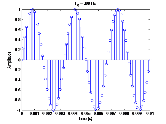
n = 0:80;
signal =
sin(2*pi()*300/8000*n);
stem(n/8000,signal);
ylabel('Amplitude')
xlabel('Time (s)')
title('F_0 = 300 Hz')
b) 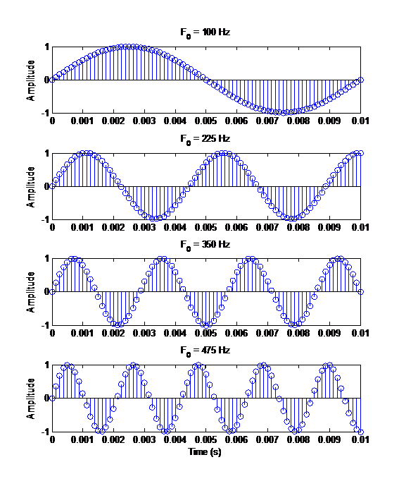
n = 0:80;
signal =
sin(2*pi()*100/8000*n);
subplot(4,1,1);
stem(n/8000,signal);
ylabel('Amplitude')
title('F_0 = 100 Hz')
signal =
sin(2*pi()*225/8000*n);
subplot(4,1,2);
stem(n/8000,signal);
ylabel('Amplitude')
title('F_0 = 225 Hz')
signal =
sin(2*pi()*350/8000*n);
subplot(4,1,3);
stem(n/8000,signal);
ylabel('Amplitude')
title('F_0 = 350 Hz')
signal =
sin(2*pi()*475/8000*n);
subplot(4,1,4);
stem(n/8000,signal);
ylabel('Amplitude')
xlabel('Time (s)')
title('F_0 = 475 Hz')
c)
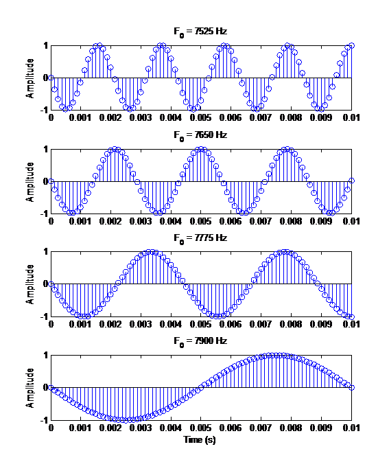
n = 0:80;
signal =
sin(2*pi()*7525/8000*n);
subplot(4,1,1);
stem(n/8000,signal);
title('F_0 = 7525
Hz')
ylabel('Amplitude')
signal =
sin(2*pi()*7650/8000*n);
subplot(4,1,2);
stem(n/8000,signal);
ylabel('Amplitude')
title('F_0 = 7650
Hz')
signal =
sin(2*pi()*7775/8000*n);
subplot(4,1,3);
stem(n/8000,signal);
ylabel('Amplitude')
title('F_0 = 7775
Hz')
signal =
sin(2*pi()*7900/8000*n);
subplot(4,1,4);
stem(n/8000,signal);
title('F_0 = 7900
Hz')
ylabel('Amplitude')
xlabel('Time (s)')
We observe that the apparent frequency decreases as the frequency of the sinusoidal increases. It has the opposite trend of part B. This must be the result of aliasing. Aliasing is expected because Fs = 8000 Hz is no longer twice the frequency of the sampled sinusoidal.
d)

n = 0:80;
signal =
sin(2*pi()*32100/8000*n);
subplot(4,1,1);
stem(n/8000,signal);
title('F_0 = 32100
Hz')
ylabel('Amplitude')
signal =
sin(2*pi()*32225/8000*n);
subplot(4,1,2);
stem(n/8000,signal);
title('F_0 = 32225
Hz')
ylabel('Amplitude')
signal =
sin(2*pi()*32350/8000*n);
subplot(4,1,3);
stem(n/8000,signal);
title('F_0 = 32350
Hz')
ylabel('Amplitude')
signal =
sin(2*pi()*32475/8000*n);
subplot(4,1,4);
stem(n/8000,signal);
title('F_0 = 32475
Hz')
ylabel('Amplitude')
xlabel('Time (s)')
We observe that the apparent frequency increases as the frequency of the sinusoidal increases. It has the same trend of part B, and in fact is identical! This must be the result of aliasing. Aliasing is expected because Fs = 8000 Hz is no longer twice the frequency of the sampled sinusoidal.
Part 2:
a) Plugging into the equation for the instantaneous frequency, we find a range of 4 kHz up to 34 kHz.
b)
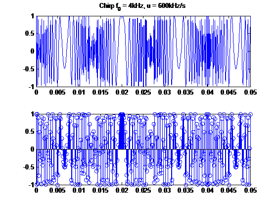
t_continuous =
0:1/8000:.05;
t =
0:1/8000:.05;
signal_continuous
= chirp(t_continuous,4000,.05,34000);
signal =
chirp(t,4000,.05,34000);
subplot(2,1,1);
plot(t_continuous,signal_continuous);
title('Chirp f_0 =
4kHz, u = 600kHz/s');
subplot(2,1,2);
stem(t,signal);
Yes there is aliasing and it starts immediately, continuing throughout the entire range calculated in part A. Aliasing is expected because Fs = 8000 Hz is never twice the frequency of the sampled sinusoidal. Although we were expecting to observe a sinusoidal with increasing frequency, our observation is of a periodic signal as a result of aliasing.
c)
The apparent frequency of the aliased signal passes through zero when the frequency of the signal passes through integer multiples of the sample frequency. Using the μ = 600 kHz/s rate and starting at 4 kHz, we can calculate all of the occurrences in the first 50 ms.
|
Signal Frequency (kHz) |
Time (ms) |
|
8 |
6.67 |
|
16 |
20 |
|
24 |
33.33 |
|
32 |
46.67 |
Part 3:
a)
clear all
t = 0:.001:2;
signal1 =
sin(2*pi()*100*t(1:400));
signal2 =
sin(2*pi()*225*t(401:800));
signal3 =
sin(2*pi()*350*t(801:1200));
signal4 =
sin(2*pi()*400*t(1201:1600));
signal5 =
sin(2*pi()*450*t(1601:length(t)));
signal =
[signal1 signal2 signal3 signal4 signal5]
plot(t,signal);
b)
The signal goes through an alias at each 5 multiple integer of 8 kHz. Thus to achieve 5 crossings, the signal must reach 40 kHz in the allotted 2 s. This results in rate of μ = (40-4)/2 = 18 kHz/s.
Part 4:
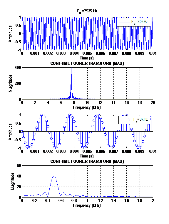
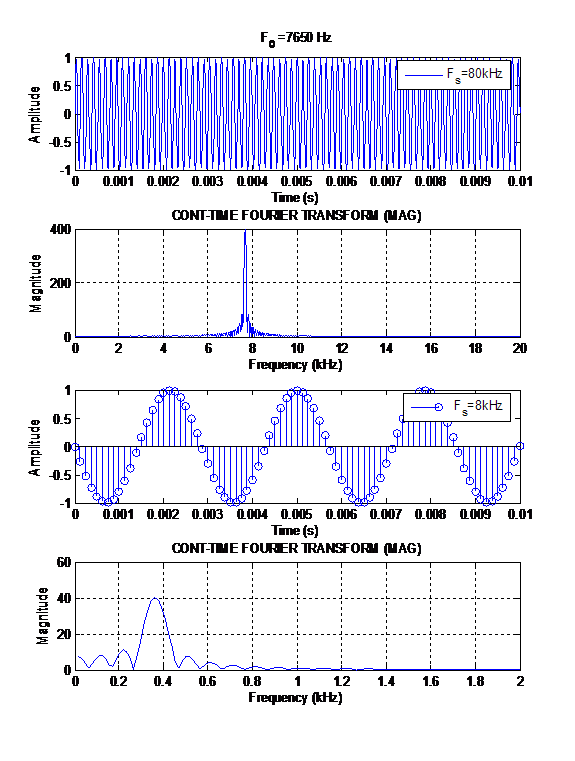


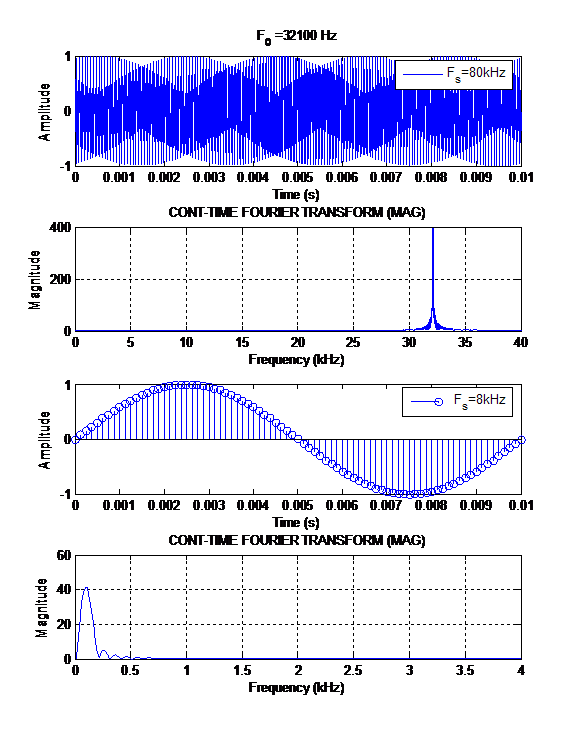
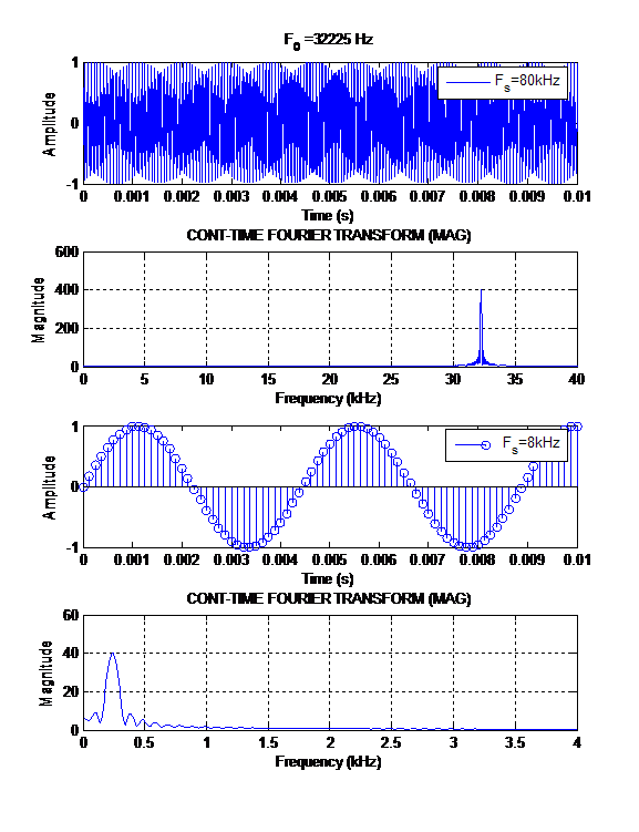
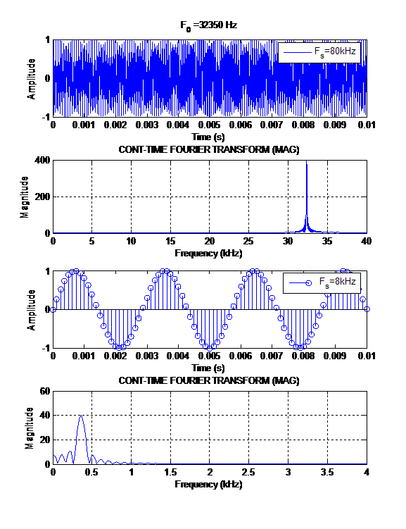
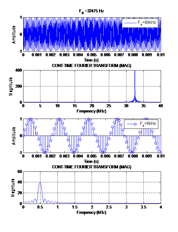
function task5(f)
n=0:800;
signal =
sin(2*pi()*f/80000*n);
subplot(411);
plot(n/80000,signal);
legend('F_s=80kHz');
title(strcat('F_0 = ',num2str(f),' Hz'));
ylabel('Amplitude')
xlabel('Time (s)')
subplot(412);
fmagplot(signal,
1/80000);
ylabel('Magnitude')
n = 0:80;
signal =
sin(2*pi()*f/8000*n);
subplot(413);
stem(n/8000,signal);
legend('F_s=8kHz');
ylabel('Amplitude')
xlabel('Time (s)')
subplot(414);
fmagplot(signal,
1/8000);
ylabel('Magnitude')