Engineering 71 Digital Signal Processing

Engineering 71 Digital Signal Processing

Lab 4 Anticausal Filtering

Mark Piper, David Luong, Brian Park, Aron Dobos

13 February 2006

Part 1: Response of Causal Filter

nn = -64:63;

unit_impulse = (nn==0);

unit_step = (nn>=0);

b = [1 0];

a = [1 -0.77];

y = filter(b, a, unit_impulse);

plot(nn, y)

title('Lab 4 Part 1, Impulse Response of H(z)=1/(1-0.77z^{-1})')

xlabel('n');

ylabel('amplitude')

y2 = filter(b,a, unit_step);

plot(nn, y2)

title('Lab 4 Part 1, Step Response of H(z)=1/(1-0.77z^{-1})')

xlabel('n');

ylabel('amplitude')

Comparison to Theoretical Discrete Response

X = tf(b,a,1);

impulse(X)

step(X)

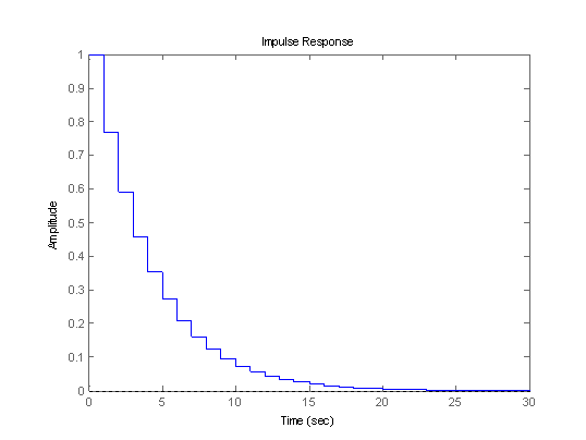
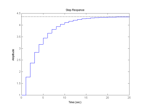
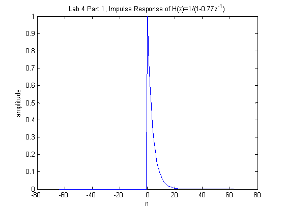
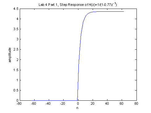
The theoretical filter response generated by MATLAB seems to agree with the result from using the ’filter’ function.

Part 2: Anticausal Filtering

A generic MATLAB function to perform anticausal filtering given transfer function polynomials B(1/z) and A(1/z) is presented below.

function [y] = filtrev(B, A, x)

xrev = fliplr(x);

yrev = filter(B,A,xrev);

y = fliplr(yrev);

We rewrite the z-domain transfer function of the filter in terms of z^-1 to determine the B and A polynomials for the causal form of the filter, to allow us to use the procedure shown above.

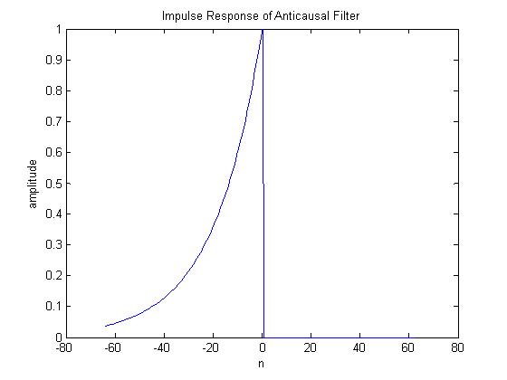
Thus, B = [ 1 0 ] and A = [ 1 -0.95 ]. Using the filtrev function, and a unit impulse, we can determine the unit impulse response of the anticausal filter.

B = [1 0];

A = [1 -0.95];

n =-64:63;

imp = (n==0);

y = fliplr( filter(B,A, fliplr(imp)) );

plot(n,y)

title('Impulse Response of Anticausal Filter')

xlabel('n');

ylabel('amplitude');

A MATLAB function was written to perform the coefficient reversal and filtering for a filter defined in its anticausal form. The generic function is given below. The derivation of the approach is also given for reference.

To convert the anticausal filter transfer function into a causal one that can be used with the filter command, we replace z with z^-1, and arrange the result into positive powers of z. A generic anticausal transfer has the form

Performing the transform , we get

Assuming the case that m = n, we rewrite H(z^-1) in positive powers of z.

Thus it is clear that the causal version of the anticausal transfer function is obtained by reversing the order of coefficients of the B and A polynomials. In the MATLAB code it must be ensured that the B and A vectors are of the same length (padded with the appropriate number of zeros to the left) so that the flip works correctly. The MATLAB code to perform this transfer function conversion and the filtering is given below.

function [y] = filtrev(B, A, x)

% function [y] = filtrev(B, A, x)

% Performs anticausal filtering on the input x by the filter

% defined in its anticausal form by B and A.

% The filtering is done by converting the causal form and

% reversing the input prior to filtering with the causal form

% and then reversing the output again.

% Written by DALU & ADOBOS1, E71 Lab 4, 15 Feb 2006

% normalize the lengths of the two vectors before

% flipping them

lenb = length(B);

lena = length(A);

len = 0;

if (lenb>lena)

len = lenb;

else

len = lena;

end

% pad the vectors

Bi = zeros(1, len);

Ai = zeros(1, len);

Bi( (len-lenb+1):len ) = B;

Ai( (len-lena+1):len ) = A;

% flip them (see derivation on paper for correctness)

Bz1 = fliplr(Bi);

Az1 = fliplr(Ai);

% perform the filtering

y = fliplr( filter(Bz1,Az1, fliplr(imp) ));

Comparison of the above data with the theoretical result shows that indeed the anticausal filter is working properly. For n>0, the impulse response is indeed zero, and it is clear that the filter is working before the input actually arrives. Therefore the filtering is indeed anticausal, as described in Proakis and Manolakis in Table 3.1 on page 159. This unfortunately cannot be verified with MATLAB’s impulse function because it only accepts causal systems.

Part 3: Cascading Causal and Noncausal Filters

clear all

close all

nn = -64:63;

unit_impulse = (nn==0);

sample=-200:200;

sin1=sin(2*pi*0.05*sample);

sin2=sin(2*pi*0.1*sample);

sin3=sin(2*pi*0.2*sample);

% Cascade Implementation with unit impulse input

h3a=filter([1 0],[1 -.77],fliplr(unit_impulse));

h3c=filter([1 0],[1 -.77],fliplr(h3a));

figure; plot(nn,h3c)

xlabel('n');

ylabel('Amplitude');

title('Unit Impulse Input');

% Cascade Implementation with 0.05Hz sinusoid

h3a=filter([1 0],[1 -.77],fliplr(sin1));

h3c=filter([1 0],[1 -.77],fliplr(h3a));

figure; plot(sample,h3c)

xlabel('n');

ylabel('Amplitude');

title('0.05Hz Sinusoid Input');

% Cascade Implementation with 0.1Hz sinusoid

h3a=filter([1 0],[1 -.77],fliplr(sin2));

h3c=filter([1 0],[1 -.77],fliplr(h3a));

figure; plot(sample,h3c)

xlabel('n');

ylabel('Amplitude');

title('0.1Hz Sinusoid Input');

% Cascade Implementation with 0.2Hz sinusoid

h3a=filter([1 0],[1 -.77],fliplr(sin3));

h3c=filter([1 0],[1 -.77],fliplr(h3a));

figure; plot(sample,h3c)

xlabel('n');

title('0.2Hz Sinusoid Input');

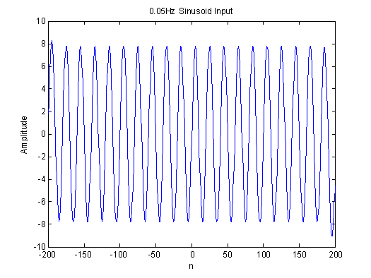
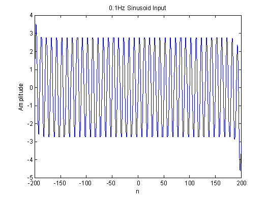
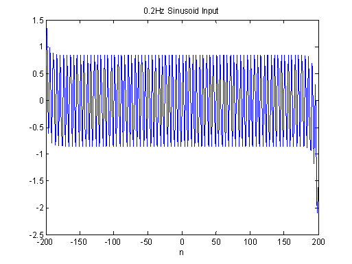
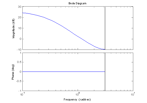
Zooming in on the zero-crossing points in the figures above, we observed no phase shift in the outputs for the tested frequencies. As a result, we suspect that this filter is a linear phase filter. The bode plot of the filter verifies our analysis:

>> H=tf([1 0],conv([-.77 1],[1 -.77]),1)

Transfer function:

-z

-------------------------

0.77 z^2 - 1.593 z + 0.77

Sampling time: 1

>> bode(H)

Part 4: Partial Fraction Expansion and Impulse Response of Cascaded Filter

clear all

close all

nn = -64:63;

unit_impulse = (nn==0);

% Parallel Implementation

beta=1.2282;

gamma=0.9457;

h4a=filter([beta gamma],[1 -.77],fliplr(unit_impulse));

h4c=filter([beta gamma],[1 -.77],unit_impulse);

h4=h4c+fliplr(h4a);

figure; plot(nn,h4)

xlabel('n');

ylabel('Amplitude');

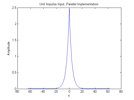
As we expected, this is the same result using the cascaded filter in Part 3.