Engineering 71 Lab 5

Brian Park, David Luong, Mark Piper, Aron Dobos

20 February 2006

Part 1: Transfer Functions

>> a2 = [ 1 -1 0 0 0 0 0 0 0 ];

>> b2 = [ 1 0 0 0 0 0 0 0 -1 ]/8;

>> s2 = tf(b2,a2,'variable','z^-1')

Transfer function:

0.125 - 0.125 z^-8

------------------

1 - z^-1

>> [y, t] = impulse(s2);

>> stem(t,y);

>> axis([0 20 0 .14])

>> xlabel('n');

>> ylabel('ampl');

>> title('Part 1 Impulse Response');

>> b1 = [ 1 1 1 1 1 1 1 1 ];

>> a1 = [ 1 0 0 0 0 0 0 0 ]*8;

>> s1 = tf(b1,a1,'variable','z^-1');

Transfer function:

1 + z^-1 + z^-2 + z^-3 + z^-4 + z^-5 + z^-6 + z^-7

--------------------------------------------------

8

b) This transfer function will average the current input with the previous 7 input values.

c) The impulse responses are the same because they are the same algebraically. The symbolic MATLAB code below confirms that this is indeed the case.

>> syms p

>> collect(simplify((1-p^-1)*(1+p^-1+p^-2+p^-3+p^-4+p^-5+p^-6+p^-7)))

ans =

1-1/p^8

d) Pole-Zero Maps using ‘pzmap’ and ‘zgrid’.

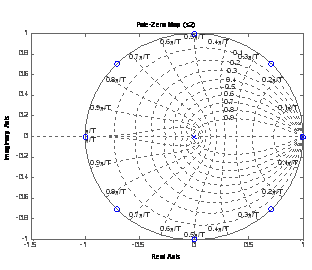
The lines made by the ‘zgrid’ command can be grouped into two categories. The lines labeled 0.1 … 0.9 indicate the damping factor of the system. Near the unit circle, the damping factor is very small, which suggests a highly oscillatory system. When the damping factor is unity, the poles are purely real, so no oscillation will result. The other lines indicate the natural frequency in terms of the sampling period T. This is because the frequency axis maps to the unit circle in the z-domain. Zero frequency is found at z = 1.

e) Explanation of PZ-Maps

All of the zeros are on the frequency axis (unit circle). Since s1 and s2 are ultimately the same transfer function algebraically, all of the poles and zeros should be the same. For s2 however, we notice a pole and zero at z = 1 that does not appear in for s1. We suggest that this pole and zero simply cancel, and that their appearance is a result of whatever mechanism MATLAB uses to plot the pole-zero maps from the transfer function.

Part 2: Frequency Domain Response of Transfer Function s2

a)

[h,w]=(freqz((b2),(a2),20));

plot(1:20,abs(h))

xlabel('n')

ylabel('amplitude')

title('Frequency Response of S2')

n = 0:100;

x1 = sin(.02*pi*n);

y1= filter(b2,a2,x1);

plot(n,x1,n,y1);

legend('x1','y1');

b)

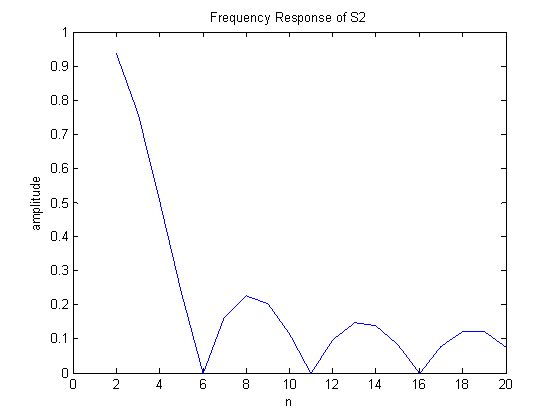
The averaging function basically acts as a low pass filter. High frequency signals tend to average to zero over our 8 data point averaging window while low frequency signals do not change much during this window and therefore do not get averaged to zero. Hence, the input mostly retains its original shape.

c)

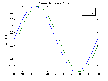
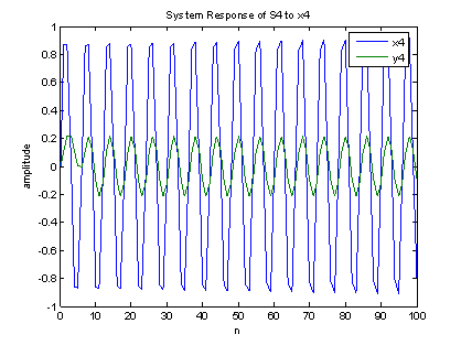
For low frequency inputs (x1), the system response acts well to pass the low frequency component as seen in the first graph. However, a slight delay is observed due to the phase shifting from the filter.

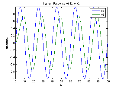
As the input frequency increases (x2), we observe the high-frequency attenuation from the low pass filter along with the delay.

In the third graph (x3), we see complete attenuation once the filter receives the required 8 samples to function. However, for a higher frequency input (x4) the filter fails to attenuate due to the side lobes of the filter response, and we observe incomplete attenuation of the input signal.

Part 3: Low pass filtering a random sequence

a)

x = rand(1000,1);

std(x)

The standard deviation is 0.2893.

b)

std(filter(b2,a2,x))

The standard deviation of the filter response is 0.1088.

c)

.2893/sqrt(8)

The actual factor is 0.1023, and matches with the result of the filtered response. We would expect the factor to be a factor of sqrt(8) less because the magnitude of the filter response is 1/sqrt(8). Since the filtered standard deviation is the product or the standard deviation of the filter and that of the input, our expectations are correct.

Part 4: Some other Matlab Commands

a)

[h,w]=(freqz((b2),(a2),20));

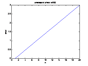
w_u = unwrap(w);

plot(1:20,w_u);

title('unwrapped phase of S2');

xlabel('n');

ylabel('ampl');

b)

syms n

pretty(ztrans( (1+n)*heaviside(n) ) );

z z

----- + --------

z - 1 2

(z - 1)

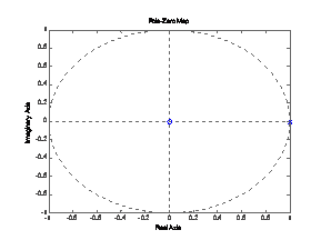
X = tf([ 1 0 0], [1 -2 1], 1);

pzmap(X)

c)

n=[1 3 0]; d=[1 3 2];

X=poly2sym(n,'z')/poly2sym(d,'z');

pretty(X)

2

z + 3 z

------------

2

z + 3 z + 2

d)

pretty(iztrans( X ))

n n

2 (-1) - (-2)

e)

DALU = ztrans( (1+n)*heaviside(n) );

pretty(diff(DALU, 'z'))

1 z 1 z

----- - -------- + -------- - 2 --------

z - 1 2 2 3

(z - 1) (z - 1) (z - 1)