Engineering 71 Lab 7
Features of Spectral Analysis
28 March 2006
David Luong, Mark Piper, Brian Park, Aron Dobos
Part 1.
close all;
Fs = 1000;
x = 0:1/Fs:2.55;
y1 = sin(2*pi*0.1*Fs*x);
y2 = sin(2*pi*1/12.8*Fs*x);
y1fft = fft(y1, 256);
y2fft = fft(y2, 256);
f = linspace(0,0.5,128);
plot( f, abs(y1fft(1:128)), f, abs(y2fft(1:128)));
title('Part 1: 256 Point FFT');
xlabel('Normalized Frequency');
ylabel('Amplitude');
y1fft = fft(y1, 1024);
y2fft = fft(y2, 1024);
f = linspace(0,0.5,512);
figure;
plot( f, abs(y1fft(1:512)), f, abs(y2fft(1:512)));
title('Part 1: 1024 Point FFT');
xlabel('Normalized Frequency');
ylabel('Amplitude');
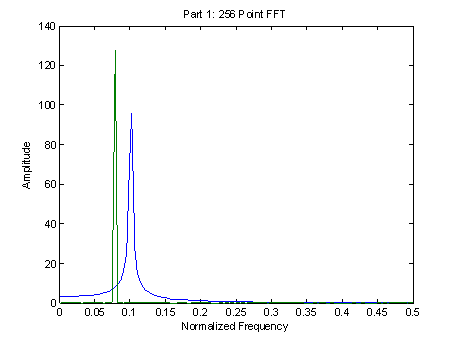
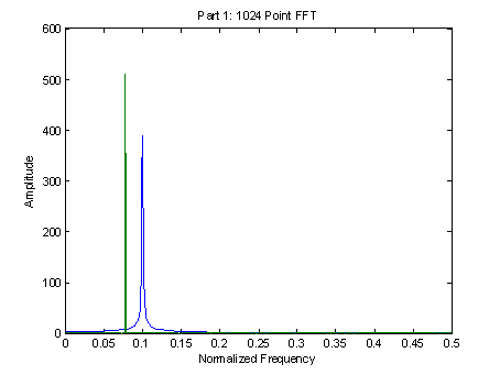
Both FFTs clearly show spikes at the expected frequencies of 0.1 and 0.0781. Although we expect that a perfect sinusoid would exhibit an impulse at the proper frequency in the frequency domain, in fact the ideal impulse is convolved in the frequency domain with the frequency response of the window. Since in time we are effectively multiplying by a square window, this results in a convolution in the frequency domain of the frequency response of the square window and the impulse, and thus gives the curved shape to the FFT result. In the 1024 point FFT, the zero padding gives a ‘better display’ of the true Fourier transform of the signal, although the spectral information is fully characterized by the 256 point FFT. It only reduces frequency estimation and scalloping errors since the Fourier transform is evaluated more densely. The difference in amplitudes between the two plots is also a result of the zero padding. Since the 1024 point FFT more closely represents the true Fourier transform (which should be an impulse for a sinusoid), it is expected that the amplitude should be larger, which it is. As a result, the amplitude scalloping error is reduced. Increasing the zero padding further results in an even higher amplitude in the frequency response for the sinusoid.
Part 2.
clear all; close all;
% Fs=100Hz, 25 data points
n=0:.01:.24;
x=sin(2*pi*10*n)+sin(2*pi*11*n);
xham=hamming(length(n))'.*(sin(2*pi*10*n)+sin(2*pi*11*n));
% Fs=100Hz, 64 fft
xfft=fft(x,64);
xhamfft=fft(xham,64);
figure; subplot(211); plot(linspace(0,0.5,32)*100,abs(xfft(1:32)));
title('25 data points, F_s=100Hz, 64 fft');
xlabel('f (Hz)'); ylabel('Amplitude');
subplot(212); plot(linspace(0,0.5,32)*100,abs(xhamfft(1:32)));
title('Hamming window, 25 data points, F_s=100Hz, 64 fft');
xlabel('f (Hz)'); ylabel('Amplitude');
% Fs=100Hz, 256 fft
xfft=fft(x,256);
xhamfft=fft(xham,256);
figure; subplot(211); plot(linspace(0,0.5,128)*100,abs(xfft(1:128)));
title('25 data points, F_s=100Hz, 256 fft');
xlabel('f (Hz)'); ylabel('Amplitude');
subplot(212); plot(linspace(0,0.5,128)*100,abs(xhamfft(1:128)));
title('Hamming window, 25 data points, F_s=100Hz, 256 fft');
xlabel('f (Hz)'); ylabel('Amplitude');
% Fs=200Hz, 50 data points
n=0:.005:.245;
x=sin(2*pi*10*n)+sin(2*pi*11*n);
xham=hamming(length(n))'.*(sin(2*pi*10*n)+sin(2*pi*11*n));
% Fs=200Hz, 64 fft
xfft=fft(x,64);
xhamfft=fft(xham,64);
figure;subplot(211);plot(linspace(0,0.5,32)*200,abs(xfft(1:32)));
title('50 data points, F_s=200Hz, 64 fft');
xlabel('f (Hz)'); ylabel('Amplitude');
subplot(212);plot(linspace(0,0.5,32)*200,abs(xhamfft(1:32)));
title('Hamming window, 50 data points, F_s=200Hz, 64 fft');
xlabel('f (Hz)'); ylabel('Amplitude');
% Fs=200Hz, 256 fft
xfft=fft(x,256);
xhamfft=fft(xham,256);
figure;subplot(211);plot(linspace(0,0.5,128)*200,abs(xfft(1:128)));
title('50 data points, F_s=200Hz, 256 fft');
xlabel('f (Hz)'); ylabel('Amplitude');
subplot(212); plot(linspace(0,0.5,128)*200,abs(xhamfft(1:128)));
title('Hamming window, 50 data points, F_s=200Hz, 256 fft');
xlabel('f (Hz)'); ylabel('Amplitude');
% Fs=100Hz, 150 data points
n=0:.01:1.49;
x=sin(2*pi*10*n)+sin(2*pi*11*n);
xham=hamming(length(n))'.*(sin(2*pi*10*n)+sin(2*pi*11*n));
% Fs=100Hz, 256 fft
xfft=fft(x,256);
xhamfft=fft(xham,256);
figure;subplot(211);plot(linspace(0,0.5,128)*100,abs(xfft(1:128)));
title('150 data points, F_s=100Hz, 256 fft');
xlabel('f (Hz)'); ylabel('Amplitude');
subplot(212);plot(linspace(0,0.5,128)*100,abs(xhamfft(1:128)));
title('Hamming window, 150 data points, F_s=100Hz, 256 fft');
xlabel('f (Hz)'); ylabel('Amplitude');
% Fs=100Hz, 512 fft
xfft=fft(x,512);
xhamfft=fft(xham,512);
figure;subplot(211);plot(linspace(0,0.5,256)*100,abs(xfft(1:256)));
title('150 data points, F_s=100Hz, 512 fft');
xlabel('f (Hz)'); ylabel('Amplitude');
subplot(212);plot(linspace(0,0.5,256)*100,abs(xhamfft(1:256)));
title('Hamming window, 150 data points, F_s=100Hz, 512 fft');
xlabel('f (Hz)'); ylabel('Amplitude');
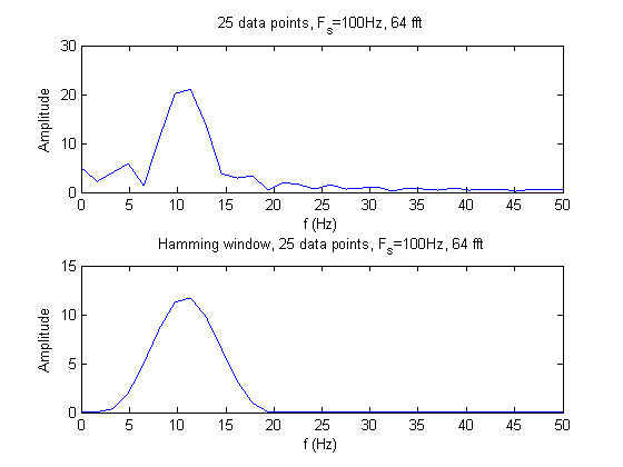
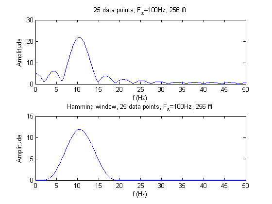
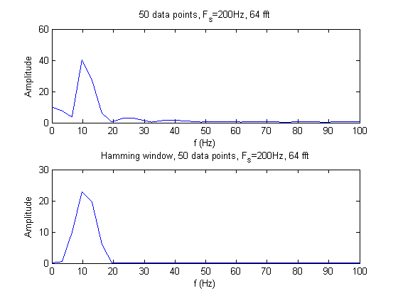
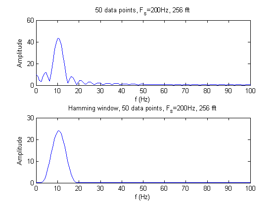
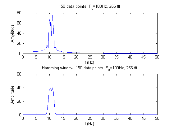
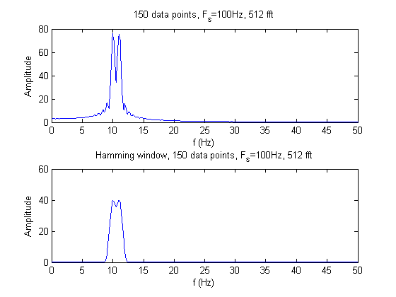
The two sinusoids can only be seen by taking 150 data points. In all other cases, the two sinusoids cannot be discernable from each other; there are not enough data points for adequate resolution. The hamming window eliminates the side lobes and decreases the noise of the signal. However, using the hamming window also decreases the dynamic range because the two sinusoids become less detectable.
Part 3.
%% part 3
Fs = 1000;
x = 0:1/Fs:5;
y1 = sin(2*pi*0.1*Fs*x);
y2 = 0.01*sin(2*pi*0.12*Fs*x);
figure;
fft1 = fft(y1+y2,256);
f = linspace(0,0.5,128);
subplot(3,1,1);
plot(f, db(abs(fft1(1:128))));
title('Part 3: 256 point FFT of 0.1 and 0.12 Sinusoids');
xlabel('Normalized Frequency');
ylabel('Amplitude (dB)');
axis([0.05 .15 -50 50])
fft2 = fft(y1+y2,512);
f = linspace(0,0.5,256);
subplot(3,1,2);
plot(f, db(abs(fft2(1:256))));
title('Part 3: 512 point FFT of 0.1 and 0.12 Sinusoids');
xlabel('Normalized Frequency');
ylabel('Amplitude (dB)');
axis([0.05 .15 -50 50])
fft3 = fft(y1+y2,1024);
f = linspace(0,0.5,512);
subplot(3,1,3);
plot(f, db(abs(fft3(1:512))));
title('Part 3: 1024 point FFT of 0.1 and 0.12 Sinusoids');
xlabel('Normalized Frequency');
ylabel('Amplitude (dB)')
axis([0.05 .15 -50 50])

Regardless of the size of the zero padding, the two sinusoids cannot be resolved with the rectangular window given their respective amplitudes. The rectangular window has the narrowest main lobe width of the various windowing functions, and as a result has the highest resolution. However, it also has large side lobes in which the second sinusoid of significantly lower amplitude remains obscured.
Part 4:
%% part 4
Fs = 1000;
x = 0:1/Fs:2.55;
y1 = sin(2*pi*0.1*Fs*x);
y2 = 0.01*sin(2*pi*0.12*Fs*x);
y = y1+y2;
w = hamming(length(y));
figure;
fft1 = fft(y.*w',256);
f = linspace(0,0.5,128);
subplot(3,1,1);
plot(f, db(abs(fft1(1:128))));
title('Part 4: 256 point fft with hamming window');
xlabel('Normalized Frequency');
ylabel('Amplitude (dB)');
axis([0.05 .15 -50 50])
fft2 = fft(y.*w',512);
f = linspace(0,0.5,256);
subplot(3,1,2);
plot(f, db(abs(fft2(1:256))));
title('Part 4: 512 point fft with hamming window');
xlabel('Normalized Frequency');
ylabel('Amplitude (dB)');
axis([0.05 .15 -50 50])
fft3 = fft(y.*w',1024);
f = linspace(0,0.5,512);
subplot(3,1,3);
plot(f, db(abs(fft3(1:512))));
title('Part 4: 1024 point fft with hamming window');
xlabel('Normalized Frequency');
ylabel('Amplitude (dB)');
axis([0.05 .15 -50 50])
%% part 5: Repeat 3
Fs = 1000;
x = 0:1/Fs:5;
y1 = sin(2*pi*0.1*Fs*x);
y2 = 0.001*sin(2*pi*0.12*Fs*x);
figure;
fft1 = fft(y1+y2,256);
f = linspace(0,0.5,128);
subplot(3,1,1);
plot(f, db(abs(fft1(1:128))));
title('Part 5a: 256 point FFT of 0.1 and 0.12 Sinusoids');
xlabel('Normalized Frequency');
ylabel('Amplitude (dB)');
axis([0.05 .15 -50 50])
fft2 = fft(y1+y2,512);
f = linspace(0,0.5,256);
subplot(3,1,2);
plot(f, db(abs(fft2(1:256))));
title('Part 5a: 512 point FFT of 0.1 and 0.12 Sinusoids');
xlabel('Normalized Frequency');
ylabel('Amplitude (dB)');
axis([0.05 .15 -50 50])
fft3 = fft(y1+y2,1024);
f = linspace(0,0.5,512);
subplot(3,1,3);
plot(f, db(abs(fft3(1:512))));
title('Part 5a: 1024 point FFT of 0.1 and 0.12 Sinusoids');
xlabel('Normalized Frequency');
ylabel('Amplitude')
axis([0.05 .15 -50 50])
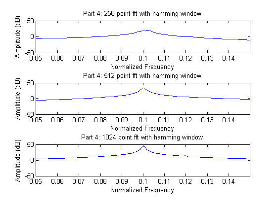
The Hamming window does not substantially improve our ability to observe both of the input sinusoids. However, relative to Part 3 where we only used a basic rectangular window, we are able to see a slight bit more activity at .12 normalized frequency when using a 1024 point FFT. This difference can be attributed to the Hamming window’s greater dynamic range. Again, the additional zero-padding of the 1024 point FFT allows for the most accurate graphic.
Part 5:
%% part 5: Repeat 4
Fs = 1000;
x = 0:1/Fs:2.55;
y1 = sin(2*pi*0.1*Fs*x);
y2 = 0.001*sin(2*pi*0.12*Fs*x);
y = y1+y2;
w = hamming(length(y));
figure;
fft1 = fft(y.*w',256);
f = linspace(0,0.5,128);
subplot(3,1,1);
plot(f, db(abs(fft1(1:128))));
title('Part 5b: 256 point fft with hamming window');
xlabel('Normalized Frequency');
ylabel('Amplitude (dB)');
axis([0.05 .15 -50 50])
fft2 = fft(y.*w',512);
f = linspace(0,0.5,256);
subplot(3,1,2);
plot(f, db(abs(fft2(1:256))));
title('Part 5b: 512 point fft with hamming window');
xlabel('Normalized Frequency');
ylabel('Amplitude (dB)');
axis([0.05 .15 -50 50])
fft3 = fft(y.*w',1024);
f = linspace(0,0.5,512);
subplot(3,1,3);
plot(f, db(abs(fft3(1:512))));
title('Part 5b: 1024 point fft with hamming window');
xlabel('Normalized Frequency');
ylabel('Amplitude (dB)');
axis([0.05 .15 -50 50])
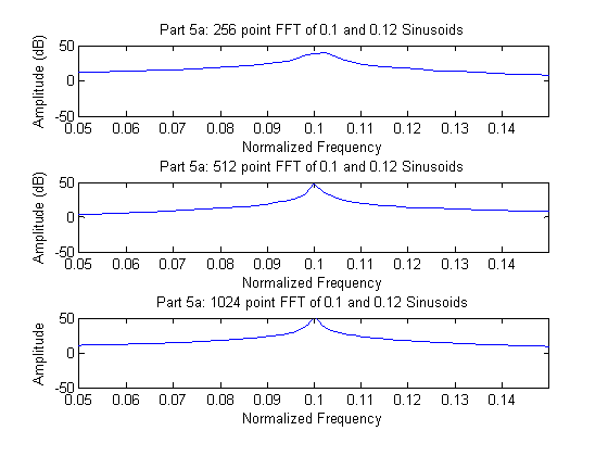
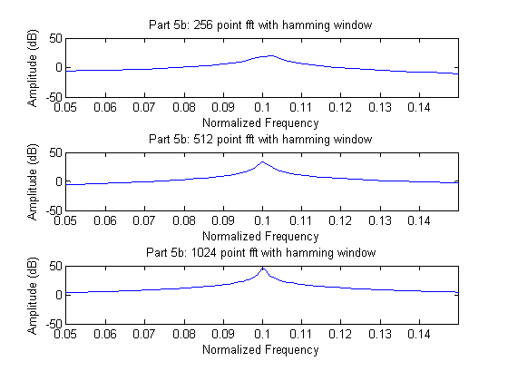
As expected, the results from part 3 and 4 only get worse as the amplitude of the smaller signal is further decreased. None of the rectangular or Hamming window attempts recognize the existence of the .12 normalized frequency component. The dynamic range discrepancy is simply to large for the windows to overcome.
Part 6:
%% part 6
Fs = 1000;
x = 0:1/Fs:2.55;
y1 = sin(2*pi*0.1*Fs*x);
y2 = 0.01*sin(2*pi*0.12*Fs*x);
for a=2:0.5:3.5,
y = y1+y2;
w = kaiser(length(y),pi*a);
figure;
fft1 = fft(y.*w',256);
f = linspace(0,0.5,128);
subplot(3,1,1);
plot(f, db(abs(fft1(1:128))));
title(sprintf('Part 6: 256 point fft with kaiser window a=%f',a));
xlabel('Normalized Frequency');
ylabel('Amplitude (dB)');
axis([0.05 .15 -50 50])
fft2 = fft(y.*w',512);
f = linspace(0,0.5,256);
subplot(3,1,2);
plot(f, db(abs(fft2(1:256))));
title(sprintf('Part 6: 512 point fft with kaiser window a=%f',a));
xlabel('Normalized Frequency');
ylabel('Amplitude (dB)');
axis([0.05 .15 -50 50])
fft3 = fft(y.*w',1024);
f = linspace(0,0.5,512);
subplot(3,1,3);
plot(f, db(abs(fft3(1:512))));
title(sprintf('Part 6: 1024 point fft with kaiser window a=%f',a));
xlabel('Normalized Frequency');
ylabel('Amplitude (dB)');
axis([0.05 .15 -50 50])
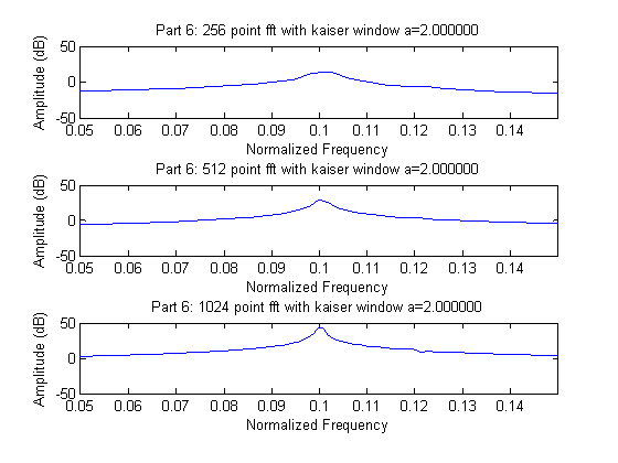
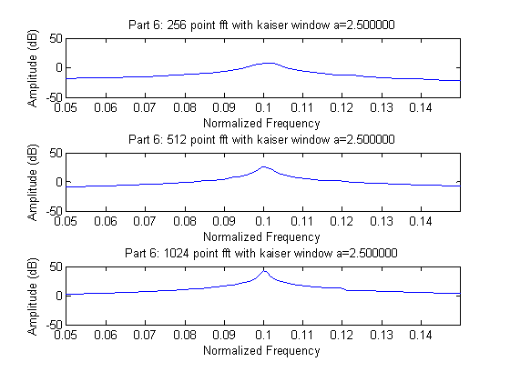
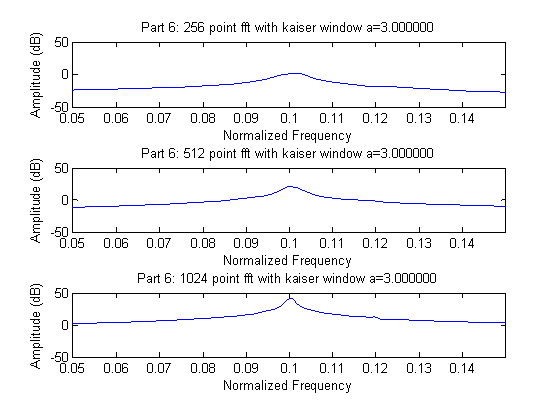
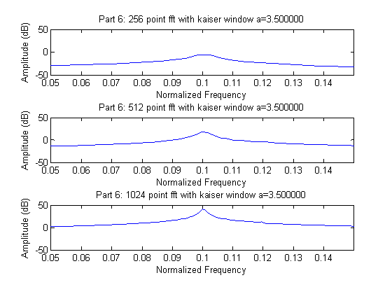
Like the Hamming window, the Kaiser-Bessel window offers a very slight improvement over the basic rectangular window. At the highest value of a, the blip at .12 becomes more defined, but still is not very prominent. These observations fit with expectation because in general the Kaiser-Bessel window offers better dynamic range than the rectangular, and at the highest level of a, has the same resolution of the rectangular. In this case the Hamming window attempts of Part 4 and the Kaiser-Bessel seem to offer comparable performance from our quick graphical analysis.