Engineering 72 Lab 7: Filters
Aron Dobos, Tyler Strombom
03 November 2004
Part 1: Op-Amp Filters

Figure 1-
The derivation for the transfer function of the op amp filter in Figure 1 is as follows
![]()
![]()


![]()

The following graphs are of our recorded data
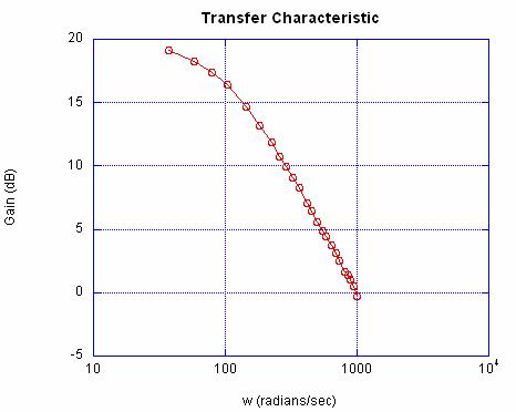
Graph 1: Gain versus Frequency
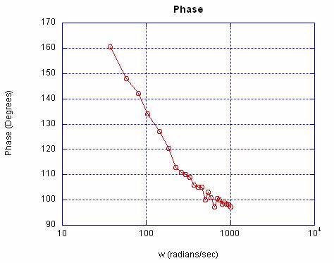
Graph 2: Phase versus Frequency
With the given values of C, R1, & R2 ![]() =100 radians/sec. From the bode plot for a “perfect” low pass
filter, (bold line on graph 3), we would expect the gain to decrease 20 dB per
decade from 100 radians/sec (
=100 radians/sec. From the bode plot for a “perfect” low pass
filter, (bold line on graph 3), we would expect the gain to decrease 20 dB per
decade from 100 radians/sec (![]() ) and a phase change of -45 degrees from 100 to 1000
radians/sec. Because a perfect low pass filter assumes exact values for
resistors and capacitors and an ideal op amp, we would not expect our data to
have these exact characteristics (thin line on graph 3).
) and a phase change of -45 degrees from 100 to 1000
radians/sec. Because a perfect low pass filter assumes exact values for
resistors and capacitors and an ideal op amp, we would not expect our data to
have these exact characteristics (thin line on graph 3).
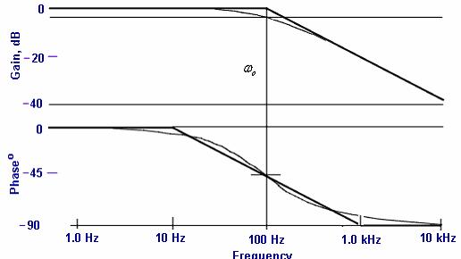
Graph 3: Bode Plots for Ideal (Bold Line) and Non Ideal (Thin line) Low Pass Filters
From http://www.oz.net/~coilgun/levitation/bodeplot.htm
Our data coincides fairly accurately with the non ideal case
in graph 3. There is a 17 dB decrease in gain from with a slight decrease in
gain before![]() . Shortly after
. Shortly after![]() , the decrease in gain is almost linear. The phase decreases
by 38 degrees from 100 to 1000 radians/sec. Around
, the decrease in gain is almost linear. The phase decreases
by 38 degrees from 100 to 1000 radians/sec. Around ![]() , the decrease in phase is fairly linear.
, the decrease in phase is fairly linear.
Part 2: Switched Capacitor Filters
The LMF100 dual switched capacitor filter IC was used to implement low, band, and high pass filter circuits. The schematic of the circuit is given below:
The forms of the transfer functions for the three filters are given below:
2nd Order High-Pass Filter: 
2nd Order Bandpass Filter: 
2nd Order Low-Pass Filter: 
By deriving the transfer function from the Mode 3 circuit schematic, we can verify that indeed the equations for f0, Q, HOLP, HOBP, and HOHP are correct.
We can derive the transfer functions for the high pass, band pass, and low pass outputs in terms of R1, R2, R3, and R4. The high pass output HPA can be arrived at by observing the following relation:

Rearranging the terms, we get the transfer function

Equating this transfer function with the form of the general high pass transfer function, we see that

![]() ,
,
 .
.
These formulas are indeed what are given in the LMF100 datasheet for f0, Q, and H0HP. The band pass and low pass transfer functions can be derived in the same way. For the band pass filter, we get:

Rearranging, we get indeed the band pass transfer function:

Equating this transfer function with the form of the general band pass transfer function, it is clear from the identical denominators that Q and f0 are the same. By manipulating some terms, we get also that the band pass gain is
![]()
which is indeed how it is given in the datasheet. To derive the low pass transfer function, we send the band pass output through another integrator. The derivation is given below.

Equating this transfer function with the form of the general low pass transfer function, it is again clear that Q and f0 remain unchanged. The low pass gain is given by
![]()
The formulas given in for f0, Q, HOLP, HOBP, and HOHP are thus shown to be correct. Given the chosen circuit component values
![]()
we calculate that
![]()
![]()

The filter was originally specified in the laboratory assignment to have a center frequency of f0 = 500 Hz, but by accident the frequency knob was bumped and only after all the measurements were made was the error realized. Instead of retaking the measurements, we assume that a filter of the above frequency was called for in the initial design. Originally, when designing the filter, we opted for a clock frequency of 50.0 kHz to give the desired 500 Hz center frequency. Plugging in values, the numerical transfer functions are
![]()
![]()
![]()
We take the magnitude of these transfer functions to
calculate the theoretical gain at various frequencies ![]() . The theoretical and
measured gains for the filters at various frequencies are listed in the table
below.
. The theoretical and
measured gains for the filters at various frequencies are listed in the table
below.
|
|
|
|
|
|
|
Freq. |
Omega |
Voltage |
Gain |
Theoretical
Gain (Matlab) |
|
36.8 |
231.2212 |
0.14 |
0.2 |
0.0087675 |
|
96.9 |
608.8406 |
0.15 |
0.214285714 |
0.06405 |
|
136 |
854.5132 |
0.17 |
0.242857143 |
0.13431 |
|
176 |
1105.841 |
0.23 |
0.328571429 |
0.24666 |
|
240 |
1507.964 |
0.45 |
0.642857143 |
0.57601 |
|
288 |
1809.557 |
0.72 |
1.028571429 |
1.0869 |
|
316 |
1985.487 |
1.07 |
1.528571429 |
1.6305 |
|
337 |
2117.433 |
1.53 |
2.185714286 |
2.2759 |
|
364 |
2287.079 |
2.35 |
3.357142857 |
3.5821 |
|
386 |
2425.309 |
2.96 |
4.228571429 |
4.7727 |
|
412 |
2588.672 |
2.95 |
4.214285714 |
4.7962 |
|
435 |
2733.186 |
2.41 |
3.442857143 |
3.948 |
|
480 |
3015.929 |
1.72 |
2.457142857 |
2.7533 |
|
541 |
3399.203 |
1.35 |
1.928571429 |
2.041 |
|
582 |
3656.814 |
1.19 |
1.7 |
1.7958 |
|
636 |
3996.106 |
1.03 |
1.471428571 |
1.5942 |
|
712 |
4473.628 |
0.96 |
1.371428571 |
1.4255 |
|
850 |
5340.707 |
0.84 |
1.2 |
1.2661 |
|
912 |
5730.265 |
0.85 |
1.214285714 |
1.2235 |
|
1058 |
6647.61 |
0.83 |
1.185714286 |
1.1573 |
|
|
|
|
|
|
|
Freq. |
Omega |
Voltage |
Gain |
Theoretical
Gain (Matlab) |
|
74.5 |
468.0973 |
0.21 |
0.3 |
0.19558 |
|
144 |
904.7787 |
0.35 |
0.5 |
0.41937 |
|
311 |
1954.071 |
0.54 |
0.771428571 |
1.919 |
|
248 |
1558.23 |
0.77 |
1.1 |
1.0165 |
|
271 |
1702.743 |
0.88 |
1.257142857 |
1.2572 |
|
310 |
1947.787 |
1.29 |
1.842857143 |
1.8967 |
|
350 |
2199.115 |
2.06 |
2.942857143 |
3.1934 |
|
372 |
2337.345 |
2.78 |
3.971428571 |
4.3013 |
|
425 |
2670.354 |
2.54 |
3.628571429 |
4.0186 |
|
458 |
2877.699 |
1.77 |
2.528571429 |
2.7826 |
|
491 |
3085.044 |
1.23 |
1.757142857 |
2.0686 |
|
531 |
3336.371 |
1.05 |
1.5 |
1.5764 |
|
582 |
3656.814 |
0.8 |
1.142857143 |
1.2179 |
|
652 |
4096.637 |
0.68 |
0.971428571 |
0.93856 |
|
712 |
4473.628 |
0.55 |
0.785714286 |
0.79023 |
|
777 |
4882.035 |
0.52 |
0.742857143 |
0.67832 |
|
868 |
5453.805 |
0.46 |
0.657142857 |
0.56953 |
|
975 |
6126.106 |
0.37 |
0.528571429 |
0.48191 |
|
1200 |
7539.822 |
0.3 |
0.428571429 |
0.36782 |
|
1473 |
9255.132 |
0.28 |
0.4 |
0.2882 |
|
|
|
|
|
|
|
Freq. |
Omega |
Voltage |
Gain |
Theoretical
Gain (Matlab) |
|
74.5 |
468.0973 |
1.2 |
1.714285714 |
1.0336 |
|
144 |
904.7787 |
1.2 |
1.714285714 |
1.1467 |
|
311 |
1954.071 |
1.3 |
1.857142857 |
2.4296 |
|
248 |
1558.23 |
1.6 |
2.285714286 |
1.6139 |
|
271 |
1702.743 |
1.2 |
1.714285714 |
1.8266 |
|
310 |
1947.787 |
1.53 |
2.185714286 |
2.4091 |
|
350 |
2199.115 |
2.29 |
3.271428571 |
3.5925 |
|
372 |
2337.345 |
2.92 |
4.171428571 |
4.5528 |
|
425 |
2670.354 |
2.36 |
3.371428571 |
3.7231 |
|
458 |
2877.699 |
1.52 |
2.171428571 |
2.3922 |
|
491 |
3085.044 |
1.05 |
1.5 |
1.6588 |
|
531 |
3336.371 |
0.77 |
1.1 |
1.1689 |
|
582 |
3656.814 |
0.56 |
0.8 |
0.82395 |
|
652 |
4096.637 |
0.39 |
0.557142857 |
0.5668 |
|
712 |
4473.628 |
0.31 |
0.442857143 |
0.43701 |
|
777 |
4882.035 |
0.26 |
0.371428571 |
0.34374 |
|
868 |
5453.805 |
0.21 |
0.3 |
0.25835 |
|
975 |
6126.106 |
0.17 |
0.242857143 |
0.19462 |
|
1200 |
7539.822 |
0.13 |
0.185714286 |
0.12069 |
|
1473 |
9255.132 |
0.11 |
0.157142857 |
0.077039 |
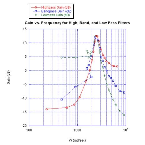
The bode plots for the measured gains for the high pass, band pass, and low pass filters are shown above. Except for a few outlier data points, the graphs show clearly the correct functioning of the three filters, despite the large peak present in all of them. Matlab generated bode plots of the filters are included below for comparison.
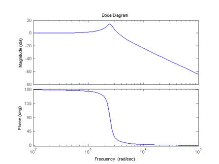
Theoretical Low-Pass Bode Plot (Matlab)

Theoretical Band-Pass Bode Plot (Matlab)
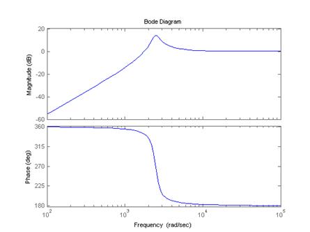
Theoretical High-Pass Bode Plot (Matlab)
Comparing the theoretical bode plots generated by Matlab for each of the given transfer functions with the measured results shows that the filters do indeed perform reasonably well.
The same measurements were repeated with the 50/100 pin on
the LMF100 pulled to V+. This change
results in a center frequency of 789.4Hz, with ![]() . The transfer
functions for the three filters with the new center frequency are given below.
. The transfer
functions for the three filters with the new center frequency are given below.
![]()
![]()
![]()
|
|
|
|
|
|
|
Freq. |
Omega |
Voltage |
Gain |
Theoretical
Gain |
|
138 |
867.079558 |
0.24 |
0.171428571 |
0.031504 |
|
220 |
1382.30074 |
0.26 |
0.185714286 |
0.084057 |
|
275 |
1727.87593 |
0.3 |
0.214285714 |
0.13769 |
|
325 |
2042.03519 |
0.36 |
0.257142857 |
0.2031 |
|
370 |
2324.77852 |
0.48 |
0.342857143 |
0.27953 |
|
440 |
2764.60149 |
0.64 |
0.457142857 |
0.44492 |
|
490 |
3078.76075 |
0.86 |
0.614285714 |
0.61441 |
|
535 |
3361.50408 |
1.1 |
0.785714286 |
0.82402 |
|
590 |
3707.07927 |
1.5 |
1.071428571 |
1.1987 |
|
660 |
4146.90223 |
2.5 |
1.785714286 |
2.0303 |
|
733 |
4605.57475 |
4.48 |
3.2 |
3.7286 |
|
755 |
4743.80483 |
5.14 |
3.671428571 |
4.368 |
|
802 |
5039.11453 |
5.88 |
4.2 |
5.0173 |
|
846 |
5315.57468 |
5.38 |
3.842857143 |
4.4043 |
|
898 |
5642.30031 |
4.32 |
3.085714286 |
3.4805 |
|
940 |
5906.19409 |
3.54 |
2.528571429 |
2.9477 |
|
1018 |
6396.28253 |
2.82 |
2.014285714 |
2.3376 |
|
1090 |
6848.67187 |
2.46 |
1.757142857 |
2.0118 |
|
1133 |
7118.84883 |
2.32 |
1.657142857 |
1.8758 |
|
1212 |
7615.22046 |
2.08 |
1.485714286 |
1.694 |
|
1288 |
8092.74254 |
1.96 |
1.4 |
1.5716 |
|
1363 |
8563.98143 |
1.86 |
1.328571429 |
1.4824 |
|
1454 |
9135.75128 |
1.76 |
1.257142857 |
1.4014 |
|
1553 |
9757.78662 |
1.76 |
1.257142857 |
1.3359 |
|
1664 |
10455.2202 |
1.68 |
1.2 |
1.2808 |
|
1734 |
10895.0431 |
1.62 |
1.157142857 |
1.2532 |
|
2037 |
12798.8483 |
1.5 |
1.071428571 |
1.1719 |
|
3250 |
20420.3519 |
1.38 |
0.985714286 |
1.0613 |
|
4115 |
25855.3071 |
1.38 |
0.985714286 |
1.0374 |
|
|
|
|
|
|
|
Freq. |
Omega |
Voltage |
Gain |
Theoretical
Gain |
|
138 |
867.079558 |
0.34 |
0.242857143 |
0.18019 |
|
220 |
1382.30074 |
0.5 |
0.357142857 |
0.30158 |
|
275 |
1727.87593 |
0.6 |
0.428571429 |
0.3952 |
|
325 |
2042.03519 |
0.72 |
0.514285714 |
0.49327 |
|
370 |
2324.77852 |
0.82 |
0.585714286 |
0.59633 |
|
440 |
2764.60149 |
1.08 |
0.771428571 |
0.79815 |
|
490 |
3078.76075 |
1.35 |
0.964285714 |
0.98972 |
|
535 |
3361.50408 |
1.58 |
1.128571429 |
1.2157 |
|
590 |
3707.07927 |
1.96 |
1.4 |
1.6037 |
|
660 |
4146.90223 |
2.98 |
2.128571429 |
2.4281 |
|
733 |
4605.57475 |
4.84 |
3.457142857 |
4.0151 |
|
755 |
4743.80483 |
5.38 |
3.842857143 |
4.5665 |
|
802 |
5039.11453 |
5.76 |
4.114285714 |
4.938 |
|
846 |
5315.57468 |
5.1 |
3.642857143 |
4.1092 |
|
898 |
5642.30031 |
3.86 |
2.757142857 |
3.0593 |
|
940 |
5906.19409 |
3 |
2.142857143 |
2.4752 |
|
1018 |
6396.28253 |
2.26 |
1.614285714 |
1.8125 |
|
1090 |
6848.67187 |
1.82 |
1.3 |
1.4568 |
|
1133 |
7118.84883 |
1.64 |
1.171428571 |
1.3068 |
|
1212 |
7615.22046 |
1.42 |
1.014285714 |
1.1032 |
|
1288 |
8092.74254 |
1.28 |
0.914285714 |
0.96313 |
|
1363 |
8563.98143 |
1.12 |
0.8 |
0.85846 |
|
1454 |
9135.75128 |
1.02 |
0.728571429 |
0.76079 |
|
1553 |
9757.78662 |
1 |
0.714285714 |
0.67898 |
|
1664 |
10455.2202 |
0.9 |
0.642857143 |
0.60757 |
|
1734 |
10895.0431 |
0.84 |
0.6 |
0.57046 |
|
2037 |
12798.8483 |
0.68 |
0.485714286 |
0.45408 |
|
3250 |
20420.3519 |
0.48 |
0.342857143 |
0.25775 |
|
4115 |
25855.3071 |
0.42 |
0.3 |
0.19899 |
|
|
|
|
|
|
|
Freq. |
Omega |
Voltage |
Gain |
Theoretical
Gain |
|
138 |
867.079558 |
1.32 |
0.942857143 |
1.0309 |
|
220 |
1382.30074 |
1.4 |
1 |
1.0822 |
|
275 |
1727.87593 |
1.42 |
1.014285714 |
1.1346 |
|
325 |
2042.03519 |
1.5 |
1.071428571 |
1.1982 |
|
370 |
2324.77852 |
1.6 |
1.142857143 |
1.2724 |
|
440 |
2764.60149 |
1.78 |
1.271428571 |
1.4321 |
|
490 |
3078.76075 |
1.96 |
1.4 |
1.5946 |
|
535 |
3361.50408 |
2.22 |
1.585714286 |
1.794 |
|
590 |
3707.07927 |
2.56 |
1.828571429 |
2.1459 |
|
660 |
4146.90223 |
3.5 |
2.5 |
2.9044 |
|
733 |
4605.57475 |
5.16 |
3.685714286 |
4.3245 |
|
755 |
4743.80483 |
5.6 |
4 |
4.7751 |
|
802 |
5039.11453 |
5.6 |
4 |
4.8609 |
|
846 |
5315.57468 |
4.76 |
3.4 |
3.8346 |
|
898 |
5642.30031 |
3.42 |
2.442857143 |
2.6895 |
|
940 |
5906.19409 |
2.52 |
1.8 |
2.0788 |
|
1018 |
6396.28253 |
1.74 |
1.242857143 |
1.4056 |
|
1090 |
6848.67187 |
1.36 |
0.971428571 |
1.0552 |
|
1133 |
7118.84883 |
1.1 |
0.785714286 |
0.9106 |
|
1212 |
7615.22046 |
0.96 |
0.685714286 |
0.7186 |
|
1288 |
8092.74254 |
0.84 |
0.6 |
0.59035 |
|
1363 |
8563.98143 |
0.68 |
0.485714286 |
0.49724 |
|
1454 |
9135.75128 |
0.64 |
0.457142857 |
0.41308 |
|
1553 |
9757.78662 |
0.6 |
0.428571429 |
0.34516 |
|
1664 |
10455.2202 |
0.5 |
0.357142857 |
0.28826 |
|
1734 |
10895.0431 |
0.48 |
0.342857143 |
0.25972 |
|
2037 |
12798.8483 |
0.36 |
0.257142857 |
0.17599 |
|
3250 |
20420.3519 |
0.26 |
0.185714286 |
0.062612 |
|
4115 |
25855.3071 |
0.24 |
0.171428571 |
0.038176 |
The bode plots for the measured gains for the high pass, band pass, and low pass filters are shown above. The graphs show clearly the correct functioning of the three filters, despite the large peak present in all of them. Matlab generated bode plots of the filters are included below for comparison.

Theoretical Low-Pass Bode Plot 2 (Matlab)
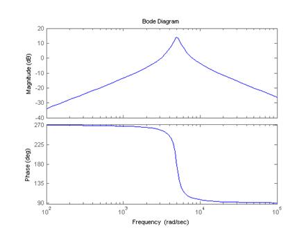
Theoretical Band-Pass Bode Plot 2 (Matlab)

Theoretical High-Pass Bode Plot 2 (Matlab)
This completes this section of the lab.
The discrete nature of the switching is clearly shown in the oscilloscope output below:
Applying a 101.5 Hz Square Wave Input
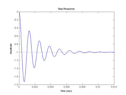
The square wave input essentially causes a step response from the system. The filter transfer functions described in great detail above control the characteristics of the various responses from the three filters. The high pass and band pass filters are all centered at 0 volts, since they do not pass low (DC) frequencies. The low pass transfer function results in a DC offset of about 0.3 volts, since some of the DC is passed.
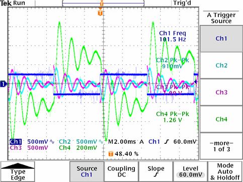
All responses to square wave.
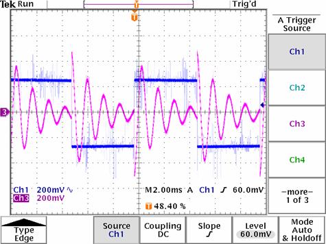
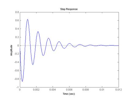
Response of band pass filter to square wave.
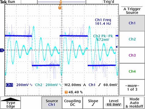
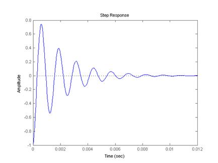
Response of high pass filter to square wave.
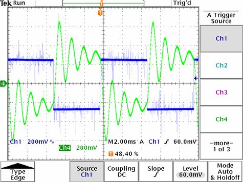
Response of low pass filter to square wave.
These results can swiftly be confirmed in Matlab. Applying a step input to each of the transfer
functions results in nearly identical waveform shapes, although the Matlab
plots assume 0 initial conditions, when clearly the initial conditions are not
zero. Since ![]() for all of the
filters, the systems are underdamped, resulting in the resonance apparent in
the oscilloscope outputs. Looking at the
high pass filter, we measure one period of the resonance to be 1.3 ms. Calculating the frequency, we get
for all of the
filters, the systems are underdamped, resulting in the resonance apparent in
the oscilloscope outputs. Looking at the
high pass filter, we measure one period of the resonance to be 1.3 ms. Calculating the frequency, we get ![]() , which is very close to the true
, which is very close to the true ![]() of 789 Hz. The
discrepancy is easily accounted for in resistor tolerances, measurement error,
and other errors. Similar calculations
could be carried out for the band pass and low pass responses. The Matlab generated step responses are
reproduced below for comparison’s sake.
of 789 Hz. The
discrepancy is easily accounted for in resistor tolerances, measurement error,
and other errors. Similar calculations
could be carried out for the band pass and low pass responses. The Matlab generated step responses are
reproduced below for comparison’s sake.