Aron Dobos
Engineering 75
17 December 2004
Time Domain Reflectometry
Introduction
Time domain reflectometry (TDR) is a way to characterize conductors that involves sending a electric pulse signal into the conductor and making measurements of the reflected signal. Reflection occurs in a variety of situations, including the interface between two different materials, an impedance change in a wire due to disfigurement or other perturbation, or any other change along the path of the transmitted pulse. The TDR is a very accurate device, and can be used in a variety of applications.
TDR was developed first in the
1950s by the power and communication industries to locate and characterize
faults in cabling. These industries
today still provide the largest target market for TDR instruments. The ability to locate disconnects and changes
in cables simplify the task of mapping out and documented cabling
installations, as well as fixing any problems.
In the 1970s, TDR technology began to be used for geological surveying
purposes by soil scientists, agricultural engineers, geotechnical engineers,
and environmental scientists. Modern oil
drilling companies are also exploiting TDR methods to accurately locate oil
deposits buried far beneath the earth surface.
TDR and radar are similar in
principle. A radar system includes a
transmitter that sends out radio frequency signals, a directional antenna, and
precise filtration and measurement systems.
The transmitted signal is simply a pulse train of radio frequency electromagnetic
energy. When the pulse hits an object,
some of the signal is reflected back, and is detected by the antenna. Knowing the elapsed time between the
transmitted and received signal, as well as the velocity of propagation of the
electromagnetic wave in the medium, the distance of the reflection interface
and be readily calculated. Sensitive
equipment can yield echo data, that when analyzed gives a detailed
characterization of not only the distance to the interface but the nature of
the interface itself. TDR works with the exact same idea.
There are traditionally two types
of TDR instruments: the waveform display, and the
digital numerical. The digital numerical
is the simpler of the types, as it only displays a calibrated number (usually
in feet or meters) corresponding to the location of the first impedance change
or discontinuity in the device under test.
Such devices are usually relatively inexpensive handheld instruments and
are useful under more restricted conditions.
The waveform display TDR shows on a LCD or CRT the graph of the
transmitted pulse and the reflections from the cable. The shape and magnitude of the reflections
can give insight into the nature of the discontinuity observed.
The rest of this paper will be
devoted to the application of TDR to transmission line cable testing.
Basic Principles
The TDR device sends a pulsed
voltage signal down a wire. Any
reflections due to glitches in the insulation, water contamination, change of
cable type, or disconnect are measured.
The width and clarity of the transmitted pulse determine the precision
of the instrument. For testing long
cables, it is necessary to send more energy down the wire so that the signal
does not die out by the time a discontinuity is reached, hence a larger pulse
width. Most instruments have settings
for pulse widths between 2ns and 1000ns to adapt to the nature of the device
under test.
Most cables are formed by two
conductors separated by a dielectric insulator.
The impedance of the cable is related to the spacing of the conductors
and the type of dielectric used. The
velocity of propagation of the electromagnetic wave down the cable is also
determined by the dielectric. The cable
type must therefore be known to accurately determine the distance of any
discontinuity.
The square pulse generated by the TDR instrument is not an instantaneous step. The finite time required to generate the pulse means that it requires a certain minimum distance along the cable to launch. A discontinuity within the minimum distance will not be clearly detected, as the pulse is not “complete” at that point along the cable. The rise time of a TDR is the time it takes for the pulse to achieve its maximum voltage value. Shorter rise times naturally result in more precise measurements, as the shape of the pulse resembles closer a brick wall energy propagation.
Mathematical Foundations
The mathematical underpinnings of TDR for cable testing can be developed from the development of a methodology and equations for transmission lines. Simple transmissions lines can be modeled as the parallel plate waveguide structure, and the electromagnetic field descriptions of the waveguide can be translated into the standard voltage, current, and impedance forms.
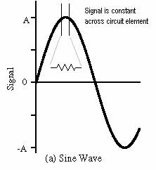
Unlike straightforward circuit elements, transmission lines cannot be modeled as lumped parameter systems. In lumped parameter circuits, it is assumed that the parameter (voltage, current) does not change across a signal circuit element – that is, the length of the component is short relative to the signal wavelength. At high frequencies or long distances, such assumptions no longer hold. Therefore,
![]() and
and
![]()
To develop equations for waves on transmission lines in terms of standard circuit parameters, we define the parameters as a function of distance along the transmission line since they are no longer constant down the entire length:
![]()
We are given the solutions for a parallel plate wave guide as
![]()
For a plate separation a and length w, we can define the voltage and the current along the waveguide as
 and
and
![]()
Applying Maxwell’s equations ![]() and
and ![]() , we arrive at what are known as the transmission line
equations
, we arrive at what are known as the transmission line
equations
![]()
where ![]() (Henrys per meter) and
(Henrys per meter) and
![]() (Farads per
meter). The characteristic impedance of
a transmission line is defined as
(Farads per
meter). The characteristic impedance of
a transmission line is defined as ![]() (ohms).
(ohms).
The following schematic shows a transmission line with characteristic impedance Z0 and a load impedance ZL.
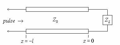
The voltage pulse sent down the transmission line can be written as the sum of the injected pulse, and any reflected wave from the load impedance. The sum appears as a forward traveling wave and a backwards traveling wave:
![]()
The reflection coefficient ![]() is defined as the
ratio of the magnitude of the backwards traveling wave to the forward traveling
wave, and thus we can write
is defined as the
ratio of the magnitude of the backwards traveling wave to the forward traveling
wave, and thus we can write
![]()
Note that this reflection coefficient is defined as the reflection at the load, hence the subscript. Given that the impedance Z(z) along the transmission line is given by
![]() ,
,
it can be seen that at z = 0, the exponential terms all go to unity. Rearranging the expression for z = 0, we obtain the reflection coefficient in terms of the load impedance.
![]()
This result is central to the principles of TDR ranging and line characterization methods. It describes how the reflection will be relative to the characteristic impedance Z0 of the line and the load impedance ZL seen the end of the line. Consider sending a voltage pulse down a transmission line. If we assume that the load impedance is infinity, that is, the cable is disconnected or broken at the end, the reflection coefficient is
![]()
This means that the reflected voltage pulse is not inverted and returns with the same magnitude as the transmitted pulse. If now the short circuit case is considered where ZL is 0, the reflection coefficient is
![]()
As such, the reflected voltage pulse will propagate backwards along the line but with a reversed sign. The magnitude of the pulse is still unchanged however. When ZL = Z0, the load impedance is matched to the line impedance, it can readily be seen that
![]()
In this “matched impedance” or “matched termination” situation, there is no reflection from the load end of the transmission line. This is desirable when electrical energy is transmitted through a power grid to distant places, since all the transmitted power ends up at the destination (the load) without reflecting back and forth along the transmission line.
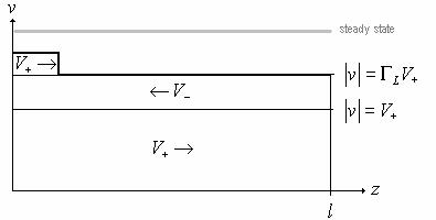
We can now consider the case of transient waves on a transmission line by looking at the response of a line to a short pulse. Consider an input pulse of the form shown below traveling down a line in the +z direction.
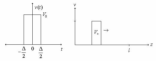
Initially, the pulse sees just the characteristic impedance of the line, as it has not yet reached the load impedance. When the pulse reaches the end of the line, it sees the load impedance ZL and reflects if the load is not perfectly matched to the line. As such, there is a pulse that
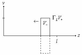
When the reflected pulse traveling backwards reaches the beginning of the transmission line, it reflects again, with again a smaller magnitude. This reflection pattern continues until the magnitude of the transient decreases to zero. Even if the reflection coefficient is unity, losses along the line will cause the transient pulses to decrease to zero.
If the injected pulse (or D.C. voltage signal) is long compared to the time it takes for it to reach the end of the line and reflect, it takes time for the line voltage to reach steady state. When the leading edge of the pulse reaches the load, it reflects, and the reflected wave is superimposed on the D.C. value of the forward traveling pulse. Eventually the magnitude of the reflection dies off and the steady state voltage as achieved on the transmission line.
The waveform display TDR instrument shows a graph of the voltage at the beginning of the transmission line as function of time. With a high speed measurement device and a short rise-time pulse generator, a TDR can be readily implemented based on the transmission line model developed above.
Oscilloscope-based TDR Implementation
A simple TDR instrument was set up in the laboratory using a high bandwidth oscilloscope and a precision pulse generator. The reflections were directly observed on the oscilloscope screen, and the reflection time was readily measured.
The pulse generator on a Tektronix TDS 8000 20GHz digital sampling oscilloscope was used to generate a fast rise-time square pulse. An SMA test cable was attached with a T-connector to a Tektronix TDS 3052 500MHz scope to view the transmission line voltage. The test cable was approximately 2 m long. The instruments are shown below:
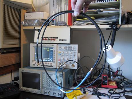
The waveform display with the test cable attached.
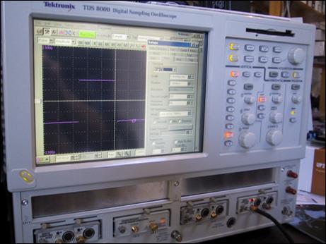
The pulse generator.

Oscilloscope
screen showing pulse and reflection in an open circuit (![]() ) configuration.
) configuration.
From the scope display the round trip time for the pulse and its reflection to arrive at the observer is measured to be 20 ns. Given the permeability and permittivity of the cable dielectric, the length of the cable can be determined. Likewise, given the cable length, the round trip time, and assuming a permeability of 1, the cable dielectric constant can be readily determined.
The cable was measured to be 1.97 m in length. The propagation velocity is given by
![]()
As a function of ![]() and
and![]() , the free space velocity is
, the free space velocity is
![]()
We can calculate the relative permittivity of the cable dielectric material as
![]()